pyyeti.cla.magpct

pyyeti.cla.magpct(M1, M2, *, Ref=None, ismax=None, symbols=None, filterval=None, plot_all=True, symlogx='auto', symlogy='auto', symlogx_range_cutoff=1000.0, symlogy_range_cutoff=500.0, ax=None)

Plot percent differences in two sets of values vs magnitude.

Parameters:

• M1, M2 (1d or 2d array_like) – The two sets of values to compare. Must have the same shape. If 2d, each column is compared.

• Ref (1d or 2d array_like or None; optional; must be named) – Same size as M1 and M2 and is used as the reference values. If None, Ref = M2.

• ismax (bool or None; optional; must be named) – If None, the sign of the percent differences is determined by M1 - M2 (the normal way). Otherwise, the sign is set to be positive where M1 is more extreme than M2. More extreme is higher if ismax is True (comparing maximums), and lower if ismax is False (comparing minimums).

• symbols (iterable or None; optional; must be named) – Plot marker iterable (eg: string, list, tuple) that specifies the marker for each column. Values in symbols are reused if necessary. For example, symbols = 'ov^'. If None, get_marker_cycle() is used to get the symbols.

• filterval (scalar, 1d array_like or None; optional; must be named) – If None, no filtering is done and all percent differences are plotted; in this case, the plot_all option is ignored. If not None, percent differences for values smaller than filterval are only plotted if plot_all is True. If they are plotted, see the symlogy argument for y-axis scaling options.

• plot_all (bool; optional; must be named) –

  Ignored if filterval is None. Otherwise:

  plot_all	Description
  True	All percent differences are plotted. The filtered region(s) will be highlighted and labeled on the plot.
  False	Plot only values larger (in the absolute sense) than filterval.

• symlogx (string or bool; optional; must be named) – Specifies whether or not to use the “symlog” option on the x-axis. This allows for a partially linear and partially logarithmic scale (see matplotlib.pyplot.xscale() for more information on the “symlog” option).

  symlogx	Description
  ‘auto’	If the range on the x-axis is greater than symlogx_range_cutoff, use the “symlog” option on the x-axis. Otherwise, keep it linear.
  True	Use the “symlog” option on the x-axis.
  False	Do not use the “symlog” option on the x-axis.

• symlogy (string or bool; optional; must be named) – Similar to the symlogx input, but treated a little differently due to the nature of the data being plotted (% differences on the y-axis vs reference magnitudes on the x-axis). If the “symlog” option is used for the y-axis, the linear range is set to the filtered values range and this region is highlighted and labeled on the plot.

  symlogy	Description
  ‘auto’	Works same as ‘auto’ for the symlogx input if filterval is None. Otherwise, if values smaller than filterval are to be plotted (see plot_all above), the “symlog” option will be used for the y-axis only if the maximum % difference for the small values is greater then twice the maximum % difference for the filtered values.
  True	Use the “symlog” option on the x-axis.
  False	Do not use the “symlog” option on the x-axis.

• symlogx_range_cutoff (scalar; optional; must be named) – Used only if symlogx == "auto"; see symlogx for description.

• symlogy_range_cutoff (scalar; optional; must be named) – Used only if symlogy == "auto" and ; see symlogx for description.

• ax (Axes object or None; must be named) – The axes to plot on. If None, ax = plt.gca().

Returns:

pdiffs (list) – List of percent differences, one 1d numpy array for each column in M1 and M2. If plot_all is True, all percent differences where M2 != 0.0 are included; otherwise, only the values above the filter are included. If M2 is all zero for a column, or all if all values are filtered out and plot_all is False, the corresponding 1d array entry in pdiffs will be zero size.

Notes

The percent differences, (M1-M2)/Ref*100, are plotted against the magnitude of Ref. If ismax is not None, signs are set as defined above so that positive percent differences indicate where M1 is more extreme than M2.

If desired, setup the plot axes before calling this routine.

This routine is called by rptpct1().

Examples

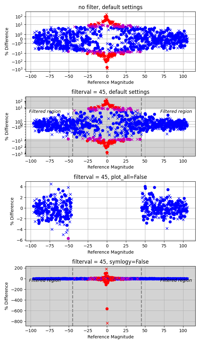
Generate some values to compare, and demo some of the options:

>>> import numpy as np
>>> import matplotlib.pyplot as plt
>>> from pyyeti import cla
>>> rng = np.random.default_rng()
>>> n = 500
>>> m1 = (
...     5 + np.arange(-n, n, 2)[:, None] / 5
...     + rng.normal(size=(n, 2))
... )
>>> m2 = m1 + rng.normal(size=(n, 2))
>>> fig = plt.figure("Example", figsize=(6.4, 11), clear=True)
>>> ax = fig.subplots(4, 1)  # , sharex=True)
>>>
>>> _ = ax[0].set_title("no filter, default settings")
>>> pdiffs = cla.magpct(m1, m2, symbols="ox", ax=ax[0])
>>>
>>> _ = ax[1].set_title("filterval = 45, default settings")
>>> pdiffs = cla.magpct(m1, m2, symbols="ox", filterval=45,
...                     ax=ax[1])
>>>
>>> _ = ax[2].set_title("filterval = 45, plot_all=False")
>>> pdiffs = cla.magpct(m1, m2, symbols="ox", filterval=45,
...                     ax=ax[2], plot_all=False)
>>>
>>> _ = ax[3].set_title("filterval = 45, symlogy=False")
>>> pdiffs = cla.magpct(m1, m2, symbols="ox", filterval=45,
...                     symlogy=False, ax=ax[3])
>>>
>>> fig.tight_layout()

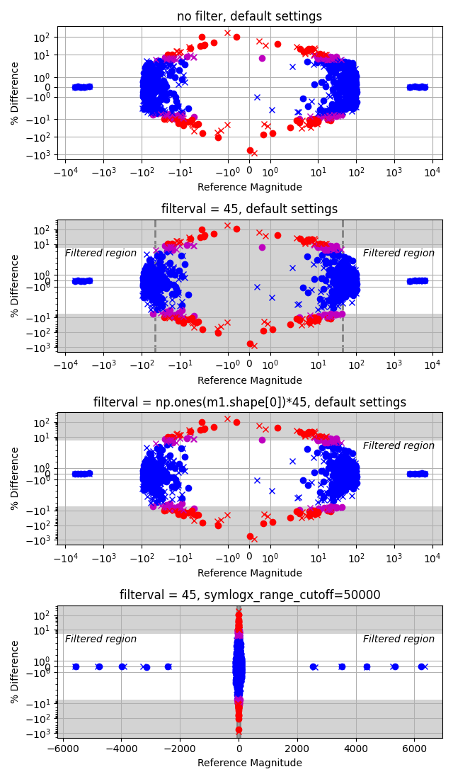
The second example will demo more options after significantly increasing the magnitude of some of the elements. Leaving the x-axis scale linear (as shown on the 4th plot) makes it difficult to see how the smaller numbers compare.

>>> m1[n - 5 :] *= np.linspace(25, 60, 5)[:, None]
>>> m2[n - 5 :] = m1[n - 5 :] + rng.normal(size=(5, 2))
>>> m1[:5] *= np.linspace(25, 60, 5)[:, None]
>>> m2[:5] = m1[:5] + rng.normal(size=(5, 2))
>>> fig = plt.figure("Example 2", figsize=(6.4, 11),
...                  clear=True)
>>> ax = fig.subplots(4, 1)
>>>
>>> _ = ax[0].set_title("no filter, default settings")
>>> pdiffs = cla.magpct(m1, m2, symbols="ox", ax=ax[0])
>>>
>>> _ = ax[1].set_title("filterval = 45, default settings")
>>> pdiffs = cla.magpct(m1, m2, symbols="ox", filterval=45,
...                     ax=ax[1])
>>>
>>> _ = ax[2].set_title("filterval = np.ones(m1.shape[0])*45"
...                     ", default settings")
>>> pdiffs = cla.magpct(m1, m2, symbols="ox",
...                     filterval=np.ones(m1.shape[0]) * 45,
...                      ax=ax[2])
>>>
>>> _ = ax[3].set_title("filterval = 45,"
...                     " symlogx_range_cutoff=50000")
>>> pdiffs = cla.magpct(m1, m2, symbols="ox", filterval=45,
...                     ax=ax[3], symlogx_range_cutoff=5e5)
>>>
>>> fig.tight_layout()