pyyeti.era.NExT

pyyeti.era.NExT(resp, sr, *, ref_channels='all', lag_start=1, lag_stop, domain='time', unbiased=True, demean=True, nperseg=None, window='hann', noverlap=None)

Use NExT method to prepare measurement data for ERA

BETA

This routine uses the “Natural Excitation Technique” to process response measurements into free-decay-like signals using auto and cross correlations. This can be done in either the time-domain or the frequency-domain. The resulting signals can then be input to ERA (the Eigensystem Realization Algorithm) for system identification. See references [1] and [2].

Parameters:

• resp (1d or 2d ndarray) – The response signal(s) to process. If 2d, each row is a response measurement. This data is expected to represent ambient vibration responses over a significant period of time. Longer measurements will result in more accurate results.

• sr (scalar) – Sample rate at which resp was sampled.

• ref_channels (integer, integer array_like, or “all”; optional) – If integer or integer array_like, specifies row(s) of resp to use as the reference channel(s) for the cross-correlations (starts at 0). Set to “all” to use all rows as reference (the default). Note that the auto-correlation of each reference channel will be included in the output.

• lag_start (integer; optional) – Cross-correlation lag for start of decay. This routine will compute auto-correlations, and for those, any noise present in the signal will be included in the 0 lag term. Specifically, the noise will be squared and summed, as if it is perfectly correlated. Therefore, the default lag_start is set to 1 to avoid including perfectly correlated noise in the decay signal.

• lag_stop (integer) – Cross-correlation lag for end of decay. It is recommended to set this to the minimum viable value based on the lowest frequency you are interested in for the current run. For example, an initial value for lag_stop might be computed such that the decay will have time for one full cycle of the estimated lowest frequency (in Hz):

  lag_stop = lag_start + sr / lowest_est_freq
  

• domain (string) – Either “time” or “frequency” to specify how this routine is to compute the cross-correlations. If “time”, scipy.signal.correlate() is used to compute the correlations using the entire time history for each cross-correlation. If “frequency”, scipy.fft.ifft() and scipy.signal.csd() are used together to compute the correlations, along with looping and windowing and averaging. If domain is “frequency”, see the inputs nperseg, window, and noverlap.

  Note

  To get the frequency domain method to give identical results to the time domain method, set nperseg to the entire signal and window to “boxcar”.

• unbiased (bool; optional) – If True, use unbiased estimates for the correlations. This should be True for ERA.

• demean (bool; optional) – If True (the default), subtract the mean from each signal prior to any other processing. Auto and cross correlations computed with demeaned signals are often called auto and cross covariances.

• nperseg (integer) – Required if domain is “frequency”. Specifies the window size to pass to scipy.signal.csd(). Generally, using higher values for nperseg will result in higher quality correlations. In order to get any benefit that might come from averaging multiple windows, a reasonable initial setting for this value might be to choose the first power-of-2 less than N / 2 where N is the number of time-steps. That would result in the largest power-of-2 size window size (for fast processing) while still giving you 3 windows to average.

• window, noverlap (optional) – These inputs are only used if domain is “frequency”. The are all passed to scipy.signal.csd(). Note that the nfft input is supplied by this routine and is set to 2 * nperseg.

Returns:

3d ndarray – Decay-like responses shaped as expected by ERA: n_channels x n_decay_tsteps x n_ref_channels. ERA will interpret the number of reference channels as the number of inputs.

References

[1]

James, G.H., Carne, T.G., and Lauffer, J.P. “The Natural Excitation Technique (NExT) for Modal Parameter Extraction From Operating Wind Turbines”, Sandia National Laboratories, Albuquerque, NM and Livermore, CA, SAND92-1666 (1993).

[2]

James, G.H., Carne, T.G., and Lauffer, J.P. “The Natural Excitation Technique (NExT) for Modal Parameter Extraction from Operating Structures”, Modal Analysis 10:260–277 (1995).

Examples

To generate synthetic ambient vibrations of a simple structure, the same system that was demoed in ERA is excited by random forces over 100 seconds. The responses are fed into NExT and then into ERA.

We have the following mass, damping and stiffness matrices (note that the damping has been specially defined to be diagonalized by the modes):

>>> import numpy as np
>>> import matplotlib.pyplot as plt
>>> import scipy.linalg as la
>>> from pyyeti import era, ode
>>> np.set_printoptions(precision=5, suppress=True)
>>>
>>> M = np.identity(3)
>>>
>>> K = np.array(
...     [
...         [4185.1498, 576.6947, 3646.8923],
...         [576.6947, 2104.9252, -28.0450],
...         [3646.8923, -28.0450, 3451.5583],
...     ]
... )
>>>
>>> D = np.array(
...     [
...         [4.96765646, 0.97182432, 4.0162425],
...         [0.97182432, 6.71403672, -0.86138453],
...         [4.0162425, -0.86138453, 4.28850828],
...     ]
... )

Since we have the system matrices, we can determine the frequencies and damping using the eigensolution.

>>> (w2, phi) = la.eigh(K, M)
>>> omega = np.sqrt(w2)
>>> freq_hz = omega / (2 * np.pi)
>>> freq_hz
array([  1.33603,   7.39083,  13.79671])
>>> modal_damping = phi.T @ D @ phi
>>> modal_damping
array([[ 0.33578, -0.     , -0.     ],
       [-0.     ,  6.9657 ,  0.     ],
       [-0.     ,  0.     ,  8.66873]])
>>> zeta = np.diag(modal_damping) / (2 * omega)
>>> zeta
array([ 0.02 ,  0.075,  0.05 ])

Simulate ambient vibrations over 100 seconds:

>>> dt = 0.01
>>> t = np.arange(0, 100, dt)
>>> n = len(t)
>>> sr = 1 / dt
>>>
>>> # for repeatability, create a specific generator:
>>> from numpy.random import Generator, PCG64DXSM
>>> rng = Generator(PCG64DXSM(seed=1))
>>> F = rng.normal(size=(3, len(t)))
>>> ts = ode.SolveUnc(M, D, K, dt)
>>> sol = ts.tsolve(force=F)

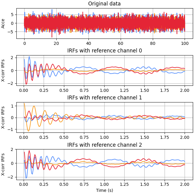
Before calling ERA, we’ll plot some auto and cross correlations directly from NExT. These should have the same properties as impulse response functions:

>>> lag_stop = 200
>>> t_irf = t[1 : lag_stop + 1]
>>> irf = era.NExT(sol.a, sr, lag_stop=lag_stop)
>>>
>>> fig = plt.figure("corr comp", clear=True, figsize=(6.4, 6.4),
...                  layout='constrained')
>>> ax = fig.subplots(4, 1)
>>>
>>> _ = ax[0].plot(t, sol.a.T)
>>> _ = ax[0].set_title("Original data")
>>> _ = ax[0].set_ylabel("Acce")
>>>
>>> # loop over all 3 ref channels:
>>> for ref in range(irf.shape[2]):
...     # loop over all 3 output channels:
...     for out in range(irf.shape[0]):
...         _ = ax[ref + 1].plot(t_irf, irf[out, :, ref])
...     _ = ax[ref + 1].set_title(f"IRFs with reference channel {ref}")
...     _ = ax[ref + 1].set_ylabel("X-corr IRFs")
>>> _ = ax[3].set_xlabel("Time (s)")

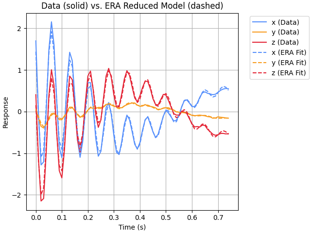
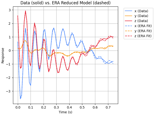
Use the time-domain method of NExT and call ERA to get estimates of frequency, damping, and mode-shapes. We’ll use a lag_stop of 75 (from sr / lowest_freq = 100 / 1.33 ~= 75).

>>> era_fit = era.ERA(
...     era.NExT(sol.a, sr, lag_stop=75),
...     sr=1 / dt,
...     auto=True,
...     input_labels=["x", "y", "z"],
...     figure_label="Time Domain ERA Fit",
... )

Current fit includes all modes:
  Mode  Freq (Hz)   % Damp    MSV     EMAC   EMACO    MPC     CMIO    MAC
  ----  ---------  --------  ------  ------  ------  ------  ------  ------
*    1     1.3307    1.5730  *0.759  *0.996  *0.997  *1.000  *0.997  *1.000
*    2     7.4842    6.4077  *0.703  *0.830  *0.928  *1.000  *0.928  *1.000
*    3    13.6264    4.7306  *1.000  *0.834  *0.928  *0.996  *0.925  *1.000
     4    14.6694    3.7619  *0.433   0.330  *0.591  *0.939  *0.555  *0.986

Auto-selected modes fit:
  Mode  Freq (Hz)   % Damp    MSV     EMAC   EMACO    MPC     CMIO    MAC
  ----  ---------  --------  ------  ------  ------  ------  ------  ------
     1     1.3307    1.5730   0.759   0.996   0.997   1.000   0.997   1.000
     2     7.4842    6.4077   0.703   0.830   0.928   1.000   0.928   1.000
     3    13.6264    4.7306   1.000   0.834   0.928   0.996   0.925   1.000

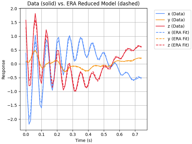
That seemed to work out pretty well! Now we’ll try the frequency-domain method of NExT (the increased svd_tol gave slightly better results in this case):

>>> era_fit = era.ERA(
...     era.NExT(
...         sol.a,
...         sr,
...         lag_stop=75,
...         domain="frequency",
...         nperseg=4096,
...     ),
...     sr=1 / dt,
...     svd_tol=0.1,
...     auto=True,
...     input_labels=["x", "y", "z"],
...     figure_label="Frequency Domain ERA Fit",
... )

Current fit includes all modes:
  Mode  Freq (Hz)   % Damp    MSV     EMAC   EMACO    MPC     CMIO    MAC
  ----  ---------  --------  ------  ------  ------  ------  ------  ------
*    1     1.3255    1.4124  *0.709  *0.994  *0.998  *1.000  *0.998  *1.000
*    2     7.4412    7.3792  *0.595  *0.750  *0.874  *0.998  *0.872  *1.000
*    3    13.7890    4.9684  *1.000  *0.499  *0.714  *1.000  *0.714  *0.999

Auto-selected modes fit:
  Mode  Freq (Hz)   % Damp    MSV     EMAC   EMACO    MPC     CMIO    MAC
  ----  ---------  --------  ------  ------  ------  ------  ------  ------
     1     1.3255    1.4124   0.709   0.994   0.998   1.000   0.998   1.000
     2     7.4412    7.3792   0.595   0.750   0.874   0.998   0.872   1.000
     3    13.7890    4.9684   1.000   0.499   0.714   1.000   0.714   0.999

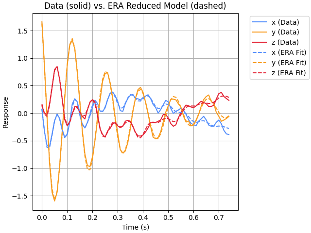
Both of the above examples used all channels as reference channels. The next example uses just the first measurement as the reference channel (which also means that the only auto-correlation that will be included will be for the first measurement):

>>> era_fit = era.ERA(
...     era.NExT(sol.a, sr, lag_stop=75, ref_channels=0),
...     sr=1 / dt,
...     auto=True,
...     input_labels=["x", "y", "z"],
...     figure_label="Time Domain ERA Fit",
... )

Current fit includes all modes:
  Mode  Freq (Hz)   % Damp    MSV     EMAC   EMACO    MPC     CMIO    MAC
  ----  ---------  --------  ------  ------  ------  ------  ------  ------
*    1     1.3309    1.6375  *0.951  *0.992  *0.993  *1.000  *0.993  *1.000
*    2    13.7399    5.1329  *1.000  *0.562  *0.750  *0.998  *0.749  *1.000

Auto-selected modes fit:
  Mode  Freq (Hz)   % Damp    MSV     EMAC   EMACO    MPC     CMIO    MAC
  ----  ---------  --------  ------  ------  ------  ------  ------  ------
     1     1.3309    1.6375   0.951   0.992   0.993   1.000   0.993   1.000
     2    13.7399    5.1329   1.000   0.562   0.750   0.998   0.749   1.000

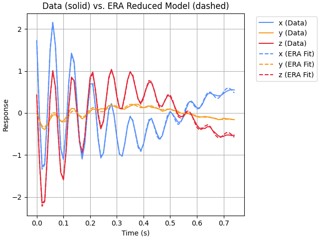
In that case, the 7.4 Hz mode was not identified. From the plot, a decent fit was found without it since the 7.x Hz content is not visibly prominent. To successfully identify that mode, it would be best to add more reference channels.