Using cb.cbcheck to check mass and stiffness
This and other jupyter notebooks are available here: https://github.com/twmacro/pyyeti/tree/master/docs/tutorials.
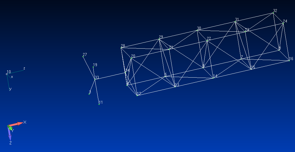
First, we need a valid Hurty-Craig-Bampton model to work with. Specifically, we need:
a-set mass and stiffness
b-set “uset” table (see description in op2.rdnas2cam)
Note: this is only needed for statically indeterminate interfaces
b-set partition vector (relative to a-set)
We’ll use superelement 102 from the test directory: “tests/nas2cam_csuper”.
Aside:
“nas2cam” stood for Nastran-to-CAM … CAM is now replaced with Python but the Nastran DMAP retains the old name.
First, do some imports:
import numpy as np
from io import StringIO
from pyyeti import nastran, cb
from pyyeti.nastran import op4
Need path to data files:
import os
import inspect
pth = os.path.dirname(inspect.getfile(cb))
pth = os.path.join(pth, 'tests', 'nas2cam_csuper')
Load the mass and stiffness from the .op4 file
This loads the data into a dict:
mk = op4.load(os.path.join(pth, 'inboard.op4'))
mk.keys()
odict_keys(['kxx', 'mxx', 'bxx1', 'k4xx1', 'px1', 'gpxx', 'gdxx', 'rvax', 'va', 'mug1', 'mug1o', 'mes1', 'mes1o', 'mee1', 'mee1o', 'mgpfm', 'mgpfb', 'mgpfk', 'mgpfo', 'mef1', 'mef1o', 'mqgm', 'mqgb', 'mqgk', 'mqg1o', 'mqmgm', 'mqmgb', 'mqmgk', 'mqmg1o'])
maa = mk['mxx'][0]
kaa = mk['kxx'][0]
Get the USET table
The USET table has the boundary DOF information (id, location, coordinate system). This is needed for superelements with an indeterminate interface. The nastran module has the function asm2uset (from nastran.bulk, actually) which is handy for forming the USET table from bulk data.
uset, coords, bset = nastran.asm2uset(os.path.join(pth, 'inboard.asm'))
# show the coordinates (which are in basic):
uset.loc[(slice(None), 1), :]
| nasset | x | y | z | ||
|---|---|---|---|---|---|
| id | dof | ||||
| 3 | 1 | 2097154 | 600.0 | 0.0 | 300.0 |
| 11 | 1 | 2097154 | 600.0 | 300.0 | 300.0 |
| 19 | 1 | 2097154 | 600.0 | 300.0 | 0.0 |
| 27 | 1 | 2097154 | 600.0 | 0.0 | 0.0 |
Form-index style b-set partition vector into a-set
We already have bset, which is a boolean partition vector for the
b-set:
bset
array([ True,  True,  True,  True,  True,  True,  True,  True,  True,
        True,  True,  True,  True,  True,  True,  True,  True,  True,
        True,  True,  True,  True,  True,  True, False, False, False,
       False, False, False, False, False], dtype=bool)
Convert to index-style for cbcheck:
b = bset.nonzero()[0]
b
array([ 0,  1,  2,  3,  4,  5,  6,  7,  8,  9, 10, 11, 12, 13, 14, 15, 16,
       17, 18, 19, 20, 21, 22, 23])
Run cbcheck
Write to a string so we can look at the output a section at a time. The
em_filt option filters the effective mass table print to only modes
with 2% or higher values.
with StringIO() as f:
    chk = cb.cbcheck(f, maa, kaa, b, b[:6], uset, em_filt=2)
    output = f.getvalue().splitlines()
lines = output[:]
Iteration 1 completed
Convergence: 4 of 6, tolerance range after 2 iterations is [8.182691848294101e-10, 1.8140751429714126e-05]
Convergence: 6 of 6, tolerance range after 3 iterations is [1.9250378964386486e-12, 2.6983748323338855e-11]
First, a note on possible output from cbcheck about iterations and convergence. That is information from the “subspace iteration” eigensolver pyyeti.ytools.eig_si. That routine is called to clean up the lowest frequency modes that are computed by scipy.la.eigh – which can be slightly off. That output is not produced for this case, since a more general eigensolver is called; this is because (as we’ll see) the mass fails the positive-definite check and the stiffness fails the symmetry check.
Before going through the text output of cbcheck, let’s take a quick look at the SimpleNamespace that it returns:
from pyyeti.pp import PP
PP(chk)
<class 'types.SimpleNamespace'>[n=10]
    .m              : float64 ndarray 1024 elems: (32, 32)
    .k              : float64 ndarray 1024 elems: (32, 32)
    .bset           : int64 ndarray 24 elems: (24,)
    .rbs            : float64 ndarray 192 elems: (32, 6)
    .rbg            : float64 ndarray 144 elems: (24, 6)
    .rbe            : float64 ndarray 192 elems: (32, 6)
    .uset           : pandas DataFrame: (24, 4)
    .effmass        : pandas DataFrame: (8, 6)
    .effmass_percent: pandas DataFrame: (8, 6)
    .cb_frq         : float64 ndarray 8 elems: (8,) [   6.12934551    6.13 <...>   281.94904595  424.81380598]
<pyyeti.pp.PP at 0x791f8a2aee10>
The SimpleNamespace contains the reordered and converted versions of the
inputs, three different sets of rigid-body modes (stiffness-based,
eigenvalue-based, and geometry-based), the Hurty-Craig-Bampton fixed
base frequencies (Hz), and some modal effective mass tables (one in mass
units, the other in percent of total). The documentation below will
cover some of these items in more detail. The following shows the
.effmass_percent DataFrame for this model. The first mode contains
31.9% of the mass in the ‘T2’ direction and 63.7% of the inertia about
the ‘R3’ axis. It also has no mass moving in the ‘T1’ direction. You can
compare the DataFrame shown to the values printed in the text output at
the end of this tutorial.
Note: A zero modal effective mass value actually just means that the masses sum to zero in that direction for that mode; which is always the case for flexible (non-rigid) free-free modes.
chk.effmass_percent
| T1 | T2 | T3 | R1 | R2 | R3 | |
|---|---|---|---|---|---|---|
| Frq (Hz) | ||||||
| 6.129346 | 4.263948e-22 | 3.192650e+01 | 6.062466e+00 | 22.622180 | 12.096581 | 63.679236 |
| 6.130134 | 1.191902e-21 | 6.064688e+00 | 3.193021e+01 | 3.493506 | 63.676216 | 12.092146 |
| 23.631877 | 2.593727e-04 | 1.747014e-23 | 8.146329e-25 | 25.133696 | 0.000004 | 0.000004 |
| 70.510647 | 2.258256e-23 | 3.078194e+01 | 9.046811e-01 | 7.263860 | 0.385570 | 13.090706 |
| 70.791530 | 5.463248e-22 | 9.051993e-01 | 3.091302e+01 | 14.573466 | 13.143242 | 0.384697 |
| 104.808515 | 4.446573e+01 | 7.296792e-22 | 7.272231e-21 | 0.000663 | 0.761462 | 0.761462 |
| 281.949046 | 1.274425e-18 | 2.991820e-01 | 2.968974e-03 | 0.083370 | 0.001027 | 0.090367 |
| 424.813806 | 3.418328e-16 | 1.249101e-02 | 4.133089e-01 | 0.096965 | 0.114215 | 0.006029 |
We’ll now focus on the text output of cbcheck. First, we’ll define a simple printing function for cleaner output viewing:
def prt(lines, next_string):
    for n, line in enumerate(lines):
        if next_string in line:
            break
    else:
        n += 1
    print('\n'.join(lines[:n]))
    return lines[n:]
The first 13 lines contain summary information. In this case, we see a warning that the mass is not positive definite and the stiffness is not symmetric. This doesn’t necessarily mean the model is bad; it could be that it’s just a little off from perfect. Everything else is as it should be:
lines = prt(lines, 'properly restrain')
Mass matrix is symmetric.
Warning: mass matrix is not positive-definite.
    However, subspace iteration succeeded, which means the mass
    must be close to positive-definite.
Warning: stiffness matrix is not symmetric: abs-max-err = 5.96e-07

Mass values check:
    Maximum value of diag(MQQ)-1.0    =           0  (should be zero) Okay
    Maximum off-diagonal value of MQQ =           0  (should be zero) Okay

Stiffness values checks:
    Maximum value of KBB              = 3.80413e+09  (should be zero only if statically-determinate) check
    Maximum value of KBQ              =           0  (should be zero) Okay
    Maximum off-diagonal value of KQQ =           0  (should be zero) Okay
    Minimum diagonal value of KQQ     =     1483.16  (should be > zero) Okay
Since the stiffness didn’t pass the symmetry check, it’s worthwhile to print a check value. Comparing this value to the maximum KBB value (above) shows that the stiffness is very close to symmetric:
abs(kaa-kaa.T).max()
5.9604644775390625e-07
Next, for statically-indeterminate models, there is a check to see if
the bref DOF properly restrain rigid-body motion. This is similar to
the SUPORT card in Nastran.
For this model, the check passes. If it failed, it would say: “Check: FAIL. Assess values below before running CLA.” instead of: “Check: PASS. Values printed below for reference.”.
The only large percent differences are for numerical zeros.
lines = prt(lines, 'Stiffness-based coordinates')
Checking to see if reference DOF properly restrain rigid-body motion.
Splitting "kbb" into the "r" (reference) and "o" (other) sets, this should be zero:

    krr - kro @ inv(koo) @ kor

Check: PASS. Values printed below for reference.

"krr" is:

    [[  4.35e+05   1.58e+06  -1.58e+06  -1.59e-07  -1.10e+07  -1.10e+07]
     [  1.58e+06   9.53e+06  -9.31e+06   1.76e+07   2.05e+07   2.42e+07]
     [ -1.58e+06  -9.31e+06   9.53e+06   1.76e+07  -2.42e+07  -2.05e+07]
     [ -1.78e-07   1.76e+07   1.76e+07   3.80e+09  -3.14e+08   3.14e+08]
     [ -1.10e+07   2.05e+07  -2.42e+07  -3.14e+08   2.18e+09   1.39e+09]
     [ -1.10e+07   2.42e+07  -2.05e+07   3.14e+08   1.39e+09   2.18e+09]]

"kro @ inv(koo) @ kor" is:

    [[  4.35e+05   1.58e+06  -1.58e+06   1.33e-06  -1.10e+07  -1.10e+07]
     [  1.58e+06   9.53e+06  -9.31e+06   1.76e+07   2.05e+07   2.42e+07]
     [ -1.58e+06  -9.31e+06   9.53e+06   1.76e+07  -2.42e+07  -2.05e+07]
     [  4.44e-07   1.76e+07   1.76e+07   3.80e+09  -3.14e+08   3.14e+08]
     [ -1.10e+07   2.05e+07  -2.42e+07  -3.14e+08   2.18e+09   1.39e+09]
     [ -1.10e+07   2.42e+07  -2.05e+07   3.14e+08   1.39e+09   2.18e+09]]

and the difference is:

    [[ -3.78e-08  -2.10e-09  -1.63e-09  -1.49e-06   4.35e-06   5.52e-06]
     [ -1.86e-09   4.10e-08   1.30e-08   8.62e-06  -1.97e-06   1.64e-05]
     [  0.00e+00   1.12e-08   5.03e-08   1.12e-05  -1.55e-05   2.96e-06]
     [ -6.21e-07   5.89e-06   8.59e-06   5.53e-03  -2.18e-03   3.48e-03]
     [  4.17e-06  -2.06e-06  -1.42e-05  -1.80e-03   1.15e-02  -1.36e-03]
     [  5.38e-06   1.73e-05   1.99e-06   3.53e-03  -1.35e-03   9.74e-03]]

The percent difference is:

    [[   0.     0.    -0.  -937.6    0.     0. ]
     [   0.    -0.     0.    -0.     0.    -0. ]
     [  -0.     0.    -0.    -0.    -0.     0. ]
     [-349.7   -0.    -0.    -0.    -0.    -0. ]
     [   0.     0.    -0.    -0.    -0.     0. ]
     [   0.    -0.     0.    -0.     0.    -0. ]]
The next section shows coordinate location information as computed from the stiffness. This first node is the reference and the others are relative to that node (and in the coordinate system of that node). The largest coordinate location error is printed for inspection. Here, the error is very small.
lines = prt(lines, 'RB Translation')
Stiffness-based coordinates relative to node starting at row/col 1 (after any reordering):
  (Note: locations are in local coordinate system of the reference node.)

         Node      ID        X         Y         Z         Error
        ------  --------  --------  --------  --------   ----------
             1         3      0.00      0.00      0.00   0.0000e+00
             2        11      0.00    300.00     -0.00   2.1876e-09
             3        19     -0.00    300.00   -300.00   2.0272e-09
             4        27     -0.00      0.00   -300.00   2.4139e-09

Maximum absolute coordinate location error:  2.41391e-09 units
The next section shows checks displacements results from rigid-body motion. All three types of rigid-body modes are used. Here everything is 1.000, perfect.
lines = prt(lines, 'MASS PROPERTIES CHECKS')
RB Translation Movement Check
-- should all be 1.0s (can be 0.0 for DOF with zero stiffness):

    Node          Stiffness-based        Geometry-based        Eigenvalue-based
    ---------   -------------------    -------------------    -------------------
           3    1.000  1.000  1.000    1.000  1.000  1.000    1.000  1.000  1.000
          11    1.000  1.000  1.000    1.000  1.000  1.000    1.000  1.000  1.000
          19    1.000  1.000  1.000    1.000  1.000  1.000    1.000  1.000  1.000
          27    1.000  1.000  1.000    1.000  1.000  1.000    1.000  1.000  1.000


RB Rotation Movement Check
-- should all be 1.0s (can be 0.0 for DOF with zero stiffness):

    Node          Stiffness-based        Geometry-based        Eigenvalue-based
    ---------   -------------------    -------------------    -------------------
           3    1.000  1.000  1.000    1.000  1.000  1.000    1.000  1.000  1.000
          11    1.000  1.000  1.000    1.000  1.000  1.000    1.000  1.000  1.000
          19    1.000  1.000  1.000    1.000  1.000  1.000    1.000  1.000  1.000
          27    1.000  1.000  1.000    1.000  1.000  1.000    1.000  1.000  1.000
The next section prints the 3 6x6 mass matrices for inspection. Information derived from these is printed afterwards. Note that the geometry reference point is different from the other two (see the cbcheck input). Since we didn’t set it, the reference for the geometry-based rb modes is (0, 0, 0) in the basic system.
lines = prt(lines, 'Comparisons from mass properties')
MASS PROPERTIES CHECKS:

6x6 mass matrix from stiffness-based rb modes:

          1.7551        0.0000       -0.0000       -0.0000     -263.2578     -263.2578
          0.0000        1.7551       -0.0000      263.2578        0.0000      772.2199
         -0.0000       -0.0000        1.7551      263.2578     -772.2199       -0.0000
         -0.0000      263.2578      263.2578   114882.5343  -115832.9863   115832.9863
       -263.2578        0.0000     -772.2199  -115832.9863   747465.3910    39598.2243
       -263.2578      772.2199       -0.0000   115832.9863    39598.2243   747465.3910


6x6 mass matrix from geometry-based rb modes:

          1.7551        0.0000       -0.0000       -0.0000      263.2578     -263.2578
          0.0000        1.7551       -0.0000     -263.2578        0.0000     1825.2510
         -0.0000       -0.0000        1.7551      263.2578    -1825.2510       -0.0000
         -0.0000     -263.2578      263.2578   114882.5343  -273787.6507  -273787.6507
        263.2578        0.0000    -1825.2510  -273787.6507  2305947.9390   -39379.1078
       -263.2578     1825.2510       -0.0000  -273787.6507   -39379.1078  2305947.9390


6x6 mass matrix from eigensolution-based rb modes:

          1.7551        0.0000       -0.0000       -0.0000     -263.2578     -263.2578
          0.0000        1.7551       -0.0000      263.2578        0.0000      772.2199
         -0.0000       -0.0000        1.7551      263.2578     -772.2199        0.0000
         -0.0000      263.2578      263.2578   114882.5343  -115832.9863   115832.9863
       -263.2578        0.0000     -772.2199  -115832.9863   747465.3910    39598.2243
       -263.2578      772.2199        0.0000   115832.9863    39598.2243   747465.3910
CG location comparison is next:
lines = prt(lines, 'Radius of gyration')
Comparisons from mass properties:

    Distance to CG location from relevant reference point:

            RB-Mode from                    X               Y               Z
            ------------              ---------------------------------------------
               Stiffness               439.998351      150.000000     -150.000000
               Geometry               1039.998351      150.000000      150.000000
               Eigensolution           439.998351      150.000000     -150.000000
Radius of gyration checks are next. The radius of gyration about an axis is the radius where all the mass would be if all the mass were at a single radius. These values should make sense with your structure. If a radius is beyond your dimensions for example, you know something is wrong (yes, this has happened … due to a badly written CONM1 or CONM2 Nastran card).
lines = prt(lines, 'Stiffness-based Inertia')
Radius of gyration about X, Y, Z axes (from CG):

        RB-Mode from                    X               Y               Z
        ------------              ---------------------------------------------
           Stiffness               143.032166      458.033929      458.033929
           Geometry                143.032166      458.033929      458.033929
           Eigensolution           143.032166      458.033929      458.033929

Radius of gyration about principal axes (from CG):

        RB-Mode from                    1               2               3
        ------------              ---------------------------------------------
           Stiffness               143.032166      457.965780      458.102068
           Geometry                143.032166      457.965780      458.102068
           Eigensolution           143.032166      457.965780      458.102068
Inertia values are printed next for inspection:
lines = prt(lines, 'GROUNDING CHECKS')
Stiffness-based Inertia Matrix @ CG about X,Y,Z:

              35905.2022        0.0000       -0.0000
                  0.0000   368201.2386      109.5583
                 -0.0000      109.5583   368201.2386

    Principal Axis Moments of Inertia:

              35905.2022   368091.6803   368310.7968


Geometry-based Inertia Matrix @ CG about X,Y,Z:

              35905.2022       -0.0000        0.0000
                 -0.0000   368201.2386      109.5583
                  0.0000      109.5583   368201.2386

    Principal Axis Moments of Inertia:

              35905.2022   368091.6803   368310.7968


Eigensolution-based Inertia Matrix @ CG about X,Y,Z:

              35905.2022        0.0000        0.0000
                  0.0000   368201.2386      109.5583
                  0.0000      109.5583   368201.2386

    Principal Axis Moments of Inertia:

              35905.2022   368091.6803   368310.7968
Grounding checks are next. This is likely the largest section. This model is very clean. Note that the grounding forces for the geometry-based rigid-body modes can only include the b-set while the other two include the q-set.
If the stiffness and eigenvalue based checks are good, but the geometry one is not good, it probably means you have a mistake in your USET table (bad coordinate system, incorrect grid location, or the grids are in the wrong order).
lines = prt(lines, 'FREE-FREE MODES')
GROUNDING CHECKS:

                            K*RB using stiffness-based rb modes:
DOF                    X           Y           Z           RX          RY          RZ
-------------     --------------------------------------------------------------------
       3   1        -0.000      -0.000      -0.000      -0.000       0.000       0.000
       3   2        -0.000       0.000       0.000       0.000      -0.000       0.000
       3   3         0.000       0.000       0.000       0.000      -0.000       0.000
       3   4        -0.000       0.000       0.000       0.005      -0.002       0.003
       3   5         0.000      -0.000      -0.000      -0.002       0.012      -0.001
       3   6         0.000       0.000       0.000       0.004      -0.001       0.010
      11   1        -0.000      -0.000      -0.000      -0.000       0.000      -0.000
      11   2        -0.000      -0.000       0.000      -0.000       0.000      -0.000
      11   3         0.000       0.000      -0.000       0.000       0.000       0.000
      11   4         0.000       0.000      -0.000       0.000      -0.000       0.000
      11   5         0.000      -0.000      -0.000       0.000       0.000      -0.000
      11   6        -0.000      -0.000       0.000      -0.000       0.000      -0.000
      19   1        -0.000       0.000      -0.000       0.000       0.000      -0.000
      19   2         0.000       0.000       0.000      -0.000      -0.000       0.000
      19   3        -0.000      -0.000       0.000      -0.000       0.000      -0.000
      19   4        -0.000       0.000      -0.000      -0.000      -0.000      -0.000
      19   5        -0.000      -0.000      -0.000       0.000       0.000      -0.000
      19   6        -0.000       0.000      -0.000       0.000       0.000      -0.000
      27   1         0.000       0.000      -0.000       0.000      -0.000       0.000
      27   2         0.000       0.000      -0.000       0.000      -0.000       0.000
      27   3         0.000       0.000      -0.000       0.000      -0.000       0.000
      27   4         0.000       0.000      -0.000       0.000      -0.000      -0.000
      27   5        -0.000      -0.000      -0.000      -0.000       0.000      -0.000
      27   6         0.000      -0.000      -0.000       0.000      -0.000       0.000
  modal     1        0.000       0.000       0.000       0.000       0.000       0.000
  modal     2        0.000       0.000       0.000       0.000       0.000       0.000
  modal     3        0.000       0.000       0.000       0.000       0.000       0.000
  modal     4        0.000       0.000       0.000       0.000       0.000       0.000
  modal     5        0.000       0.000       0.000       0.000       0.000       0.000
  modal     6        0.000       0.000       0.000       0.000       0.000       0.000
  modal     7        0.000       0.000       0.000       0.000       0.000       0.000
  modal     8        0.000       0.000       0.000       0.000       0.000       0.000

Summation of stiffness-based rb-forces: RB'*K*RB:

        -0.000      -0.000      -0.000      -0.000       0.000       0.000
        -0.000       0.000       0.000       0.000      -0.000       0.000
         0.000       0.000       0.000       0.000      -0.000       0.000
        -0.000       0.000       0.000       0.005      -0.002       0.004
         0.000      -0.000      -0.000      -0.002       0.012      -0.001
         0.000       0.000       0.000       0.003      -0.001       0.010


                            K*RB using geometry-based rb modes:
DOF                    X           Y           Z           RX          RY          RZ
-------------     --------------------------------------------------------------------
       3   1        -0.000       0.000      -0.000      -0.000       0.000       0.000
       3   2        -0.000       0.000      -0.000      -0.000       0.000       0.000
       3   3         0.000      -0.000       0.000       0.000      -0.000      -0.000
       3   4        -0.000      -0.000      -0.000      -0.000       0.000      -0.001
       3   5         0.000      -0.000       0.000       0.000      -0.001      -0.003
       3   6         0.000      -0.000       0.000       0.000      -0.003      -0.001
      11   1         0.000       0.000       0.000      -0.000      -0.000       0.000
      11   2         0.000       0.000       0.000       0.000      -0.000       0.000
      11   3        -0.000      -0.000      -0.000       0.000       0.000      -0.000
      11   4         0.000       0.000       0.000      -0.000      -0.002       0.003
      11   5        -0.000      -0.000      -0.000      -0.000       0.003      -0.002
      11   6         0.000      -0.000       0.000      -0.000      -0.001      -0.000
      19   1        -0.000      -0.000       0.000       0.000      -0.000      -0.000
      19   2         0.000       0.000      -0.000       0.000       0.000       0.000
      19   3        -0.000      -0.000       0.000       0.000      -0.000      -0.000
      19   4         0.000       0.000       0.000      -0.000      -0.001       0.001
      19   5         0.000      -0.000       0.000       0.000      -0.001      -0.003
      19   6         0.000      -0.000       0.000       0.000      -0.003      -0.001
      27   1        -0.000       0.000       0.000      -0.000      -0.000       0.000
      27   2        -0.000       0.000       0.000       0.000      -0.000       0.000
      27   3        -0.000       0.000       0.000      -0.000      -0.000       0.000
      27   4        -0.000       0.000      -0.000      -0.000       0.000       0.000
      27   5        -0.000       0.000       0.000      -0.000      -0.002       0.003
      27   6        -0.000      -0.000      -0.000      -0.000       0.003      -0.002

Summation of geometry-based rb-forces: RB'*K*RB:

        -0.000      -0.000      -0.000      -0.000      -0.000       0.000
        -0.000       0.000       0.000      -0.000      -0.000       0.000
         0.000       0.000       0.000       0.000      -0.000       0.000
         0.000      -0.000       0.000       0.005      -0.006      -0.007
        -0.000      -0.000      -0.000      -0.005       0.050      -0.005
         0.000       0.000       0.000      -0.004      -0.005       0.048


                            K*RB using eigensolution-based rb modes:
DOF                    X           Y           Z           RX          RY          RZ
-------------     --------------------------------------------------------------------
       3   1        -0.000       0.000      -0.000       0.000       0.000       0.000
       3   2        -0.000       0.000      -0.000       0.000       0.000       0.000
       3   3         0.000      -0.000       0.000      -0.000      -0.000      -0.000
       3   4         0.000      -0.000      -0.000      -0.000       0.000      -0.000
       3   5         0.000      -0.000       0.000      -0.000      -0.001      -0.001
       3   6         0.000      -0.000       0.000      -0.000      -0.002      -0.001
      11   1         0.000      -0.000       0.000      -0.000      -0.000      -0.000
      11   2         0.000       0.000       0.000       0.000      -0.000       0.000
      11   3        -0.000      -0.000      -0.000      -0.000       0.000      -0.000
      11   4         0.000       0.000       0.000       0.000      -0.001       0.001
      11   5        -0.000      -0.000      -0.000      -0.000       0.002      -0.001
      11   6         0.000      -0.000       0.000      -0.000      -0.000      -0.000
      19   1        -0.000      -0.000       0.000      -0.000      -0.000      -0.000
      19   2         0.000       0.000      -0.000       0.000       0.000      -0.000
      19   3        -0.000      -0.000       0.000       0.000       0.000      -0.000
      19   4         0.000       0.000       0.000      -0.000      -0.000       0.000
      19   5        -0.000      -0.000       0.000      -0.000      -0.001      -0.001
      19   6        -0.000      -0.000       0.000       0.000      -0.002      -0.000
      27   1        -0.000       0.000       0.000       0.000      -0.000       0.000
      27   2        -0.000       0.000       0.000       0.000      -0.000       0.000
      27   3        -0.000       0.000       0.000       0.000      -0.000       0.000
      27   4        -0.000       0.000      -0.000      -0.000       0.000       0.000
      27   5         0.000       0.000       0.000       0.000      -0.001       0.001
      27   6        -0.000      -0.000      -0.000      -0.000       0.002      -0.001
  modal     1        0.000      -0.000       0.000      -0.000      -0.000      -0.000
  modal     2        0.000       0.000       0.000       0.000      -0.000       0.000
  modal     3        0.000       0.000       0.000      -0.000      -0.000      -0.000
  modal     4       -0.000       0.000       0.000       0.000       0.000       0.000
  modal     5        0.000       0.000      -0.000       0.000      -0.000      -0.000
  modal     6       -0.000       0.000      -0.000       0.000      -0.000       0.000
  modal     7       -0.000       0.000      -0.000      -0.000       0.000       0.000
  modal     8       -0.000       0.000      -0.000       0.000       0.000       0.000

Summation of eigensolution-based rb-forces: RB'*K*RB:

        -0.000      -0.000      -0.000      -0.000       0.000       0.000
        -0.000       0.000       0.000       0.000      -0.000       0.000
         0.000       0.000       0.000       0.000      -0.000       0.000
        -0.000       0.000       0.000       0.005      -0.002       0.004
         0.000      -0.000      -0.000      -0.002       0.012      -0.001
         0.000       0.000       0.000       0.003      -0.001       0.010
The free-free mode check is next. The rigid-body modes should be close to zero frequency. (I actually depend on this more than the grounding checks above to check for grounding.) As noted previously, this model is very clean.
lines = prt(lines, 'Modal Effective Mass')
FREE-FREE MODES:

    Mode   Frequency (Hz)
    ----   --------------
       1         0.000024
       2         0.000012
       3         0.000020
       4         0.000023
       5         0.000032
       6         0.000046
       7        47.926681
       8        47.985939
       9        53.273647
      10       137.646420
      11       156.953727
      12       158.291832
      13       245.776945
      14       245.776945
      15       278.650359
      16       291.228161
      17       296.280852
      18       304.217218
      19       429.385190
      20      1479.543087
      21      1509.151143
      22      1611.251104
      23      2421.562811
      24      2421.562963
      25      2520.830498
The last section prints the modal effective mass using the geometry-based rb modes. This should match the provided documentation if there is any.
lines = prt(lines, 'end of file')
FIXED-BASE MODES w/ Percent Modal Effective Mass:

Using geometry-based rb modes for effective mass calcs.

Printing only the modes with at least 2.0% effective mass.
The sum includes all modes.

Mode No.  Frequency (Hz)     T1      T2      T3      R1      R2      R3
--------  --------------   ------  ------  ------  ------  ------  ------
     1          6.129        0.00   31.93    6.06   22.62   12.10   63.68
     2          6.130        0.00    6.06   31.93    3.49   63.68   12.09
     3         23.632        0.00    0.00    0.00   25.13    0.00    0.00
     4         70.511        0.00   30.78    0.90    7.26    0.39   13.09
     5         70.792        0.00    0.91   30.91   14.57   13.14    0.38
     6        104.809       44.47    0.00    0.00    0.00    0.76    0.76

Total Effective Mass:       44.47   69.99   70.23   73.27   90.18   90.10