Eigensystem Realization Algorithm Tutorial
Many thanks to Natalie Hintz for this tutorial!
This and other jupyter notebooks are available here: https://github.com/twmacro/pyyeti/tree/master/docs/tutorials.
System realization encompasses the practice of using numerical methods to obtain a model of a system from experimental data of the system’s response to an impulse. This realization, while derived from discrete-time data, should satisfy the system’s continuous-time domain model as well. From this realization, a system’s modal data can be derived.
The Eigensystem Realization Algorithm (ERA) is a realization method used to identify a system’s modal parameters from noisy measurement data [1]. A system’s response to an impulse, such as a separation shock event, allows it to experience free decay, which contains useful frequency and modal damping information. ERA assembles impulse response data of the system into a block Hankel matrix and that matrix is manipulated to find the system modal parameters (natural frequencies, mode shapes, and damping).
The calculated modal responses produced by ERA can be reduced by a couple of means. The choice of how to arrange the system’s data block matrix can help to filter out some signal noise and focus in on true modal responses. Carefully selecting the free-decay-only data can help this process, as can adjusting the tolerance level of the ERA procedure. It is highly recommended to run ERA multiple times while tweaking the inputs to gain confidence in the results.
Additionally, there are some methods which can be used to identify system modes and differentiate them from noise. Four of these methods are used in this program, Mode Singular Value (MSV), Extended Modal Amplitude Coherence (EMAC), Modal Phase Collinearity (MPC), and Modal Amplitude Coherence (MAC). They are used in conjunction to provide more information regarding the importance of each detected mode to the approximation of the original signal.
The MSV of each mode has been normalized within this program, and so ranges from 0.0 to 1.0 with larger values indicating larger contribution of the mode to the response.
The EMAC of each mode ranges from a scale of 0.0 to 1.0, and is a temporal measure indicating the importance of the mode over time to the fit [2]. Higher values for a given mode indicate more importance to the overall response. From experience, the EMAC is superior to the MAC value (see below).
The MPC of each mode ranges from 0.0 to 1.0 and is a spatial measure indicating whether or not the different response locations for a mode are in phase. Higher values indicate more “in-phase” measurements. This method is only useful if there are multiple outputs (MPC is 1.0 for single output).
The MAC of each mode ranges from a scale of 0.0 to 1.0 and is a temporal measure indicating the importance of the mode over time to the fit, like the EMAC. A larger MAC value for a mode indicates that it plays an important role in approximating the fit of the realization model to the experimental data, while a lower value is less important and therefore more likely to be the product of noise. For our purposes, a MAC of 0.95 or higher is considered a strong indicator that a detected mode is a true system response rather than noise. The MAC value for a mode is the dot product of two vectors: (1) The ideal, reconstructed time history for a mode; (2) The time history extracted from the input data for the mode after discarding noisy data via singular value decomposition. From experience, this indicator is not as useful as the EMAC.
References:
[1] Jer-Nan Juang. Applied System Identification. United Kingdom: Prentice Hall, 1994.
[2] Richard S. Pappa, Kenny B. Elliott, Axel Schenk. “A Consistent-Mode Indicator for the Eigensystem Realization Algorithm”, NASA Technical Memorandum 107607, April 1992.
Using the ERA Class
The necessary functions to perform ERA on a set of experimental data is contained within the class ERA. It accepts 14 parameters:
Response
Sample rate
Singular value tolerance level
Automatic selection toggle
Lower limit for MSV
Lower limit for EMAC
Lower limit for MPC
Lower limit for MAC
Range of acceptable modal damping values
Initial time value
Show plot of ERA fit
Input data labels
Input data FFT display toggle
FFT display frequency range
Response (resp)
The system’s free-decay response data is provided via the parameter
‘resp’. This data may be as large as 3-dimensional, in the shape of a
n_outputs x n_tsteps x n_inputs matrix. Often n_inputs will be
equal to 1 except for special cases.
The system’s response data, once fed into the program, will be used to construct a block Hankel matrix. This block data matrix will be decomposed and used to determine the system modes.
Sample Rate (sr)
The rate at which the response data was sampled.
Singular Value Tolerance Level (svd_tol)
The tolerance level of the ERA class allows the program to detect and exclude some noise modes. The default value for this parameter is 0.01, but it can be input as an even integer or as a positive decimal less than 1.
If the tolerance input is provided as an integer, it dictates how many true modes the program should expect to find. This number should be provided as twice the number of modes expected (e.g. if there are 3 modes of interest, the tolerance would be set to 6). The program will use this value to adjust its calculations to report this number of modes back to its user.
If the tolerance input is provided as a decimal, it is used to denote how large a singular value will need to be relative to the largest singular value of the system in order to be considered relevant. If this value is too small, it can cause more noise modes to be reported. There is a safeguard against this in the class; if a tolerance level is too small, it will be loosened automatically to ensure that no ‘impossible’ modes (i.e. those with negative damping) will be reported. However, this tolerance can also be experimentally adjusted to determine the optimum value which will produce the most true modes.
This parameter is optional, with 0.01 as the default value.
Automatic vs. Interactive Modes (auto)
If the auto parameter is set to True, the ERA class will automatically execute its calculations of detected modes, then identify true modes based on the mode indicator values of each. If the mode indicator values of a given mode are greater than or equal to the lower limits set by the user, then these will be reported as true modes.
If the auto parameter is set to False, this will enable the ERA class’ interactive setting. This mode of operation will enable the user to have more input regarding which detected modes are the product of noise and which are true modes. First, all of the detected modes will be printed for the user, and the recommended modes (those which would be automatically kept) will be marked with an asterisk. The user will then be prompted to indicate whether any modes should be removed from consideration. If any modes are selected from removal, they will not be present for the remainder of the process, and their absence will be reflected in generated plots of approximated fit. After this step, the user will be able to select modes to isolate for analysis, and the class will print these modes separately from the rest, as well as plot the resulting approximated fit of the data solely using the contribution of these modes. This can be performed as many times as necessary, and the end of each mode selection will return to the full list of modes (excluding any which were initially removed).
This parameter is optional, with False as the default value.
Mode Indicator Limits (MSV_lower_limit, EMAC_lower_limit, MPC_lower_limit, MAC_lower_limit)
These four parameters correspond to the four built-in mode indicator methods of the ERA algorithm. As mentioned above, these parameters range in value from 0.0 to 1.0, with larger values generally indicating larger contribution of a mode to a response (with the exception of MPC which indicates whether response locations of a mode are in phase). These limits come into effect when the sutomatic mode of the algorithm has been enabled, as modes with mode indicator values below these limits will be identified as noise modes and removed accordingly. These parameters accept float values from 0.0 to 1.0.
These parameters are optional; their default values vary depending on the mode indicator. Please reference the ERA documentation within pyYeti to learn more.
Acceptable Damping Range (damp_range)
This parameter sets the acceptable range for modal damping values for modes automatically detected by the algorithm. These limits are inclusive.
This parameter is optional, and the default value is (0.001, 0.999).
Initial Time Value (t0)
The initial time value is only used for plotting purposes within the ERA algorithm. The value of t0 should correspond with the initial time in the system response, ‘resp’.
This parameter is optional, its default value is 0.0.
Show ERA Fit (show_plot)
This parameter, if set to True, will show a plot of the ERA fit (represented with dashed lines) against the response data (represented with solid lines).
This parameter is optional, the default value is True.
Input Signal Labeling (input_labels)
The ERA class gives its user the option to specify a list of labels for each of the processed signals. For example, if there are three signals processed by the class, corresponding to x, y, and z axes, then the user may wish to input the labels [‘x’, ‘y’, ‘z’]. This parameter allows the program to create a legend to accompany the approximated fit plot, and will label the signals and their approximations accordingly, allowing for a better understanding of the displayed data.
This parameter is optional, the default value is None.
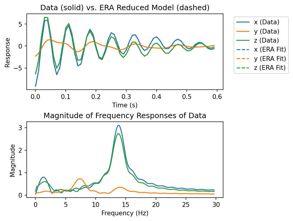
Enabling Fast Fourier Transform Plot (FFT, FFT_range)
While the Eigensystem Realization Algorithm is a reliable and resilient method of determining the modes of a response, it can be helpful to have additional verification of the program’s results. For this reason, the ERA class has the parameter ‘FFT’ which, if True, will produce an FFT plot of the data provided to the program. This plot is another tool to indicate contributing frequencies to the signal, so it should align well with the program’s detected modes.
While it may be useful to produce an FFT plot, the scaling of the plot may not be optimal to allow for visual analysis. Due to the presence of signal noise, there are likely to be many high-frequency and low amplitude peaks caught by FFT, and these will make it more difficult to see important lower frequency contributions. In this case, the parameter ‘FFT_limit’ allows for the adjustment of the x-axis to limit what frequencies are plotted. A single value will act as an upper limit to the frequencies displayed, while a pair of values will act as lower and upper cutoffs, respectively.
These parameters are optional; the default value of ‘FFT’ is False, and the default value of ‘FFT_range’ is None.
Output of the ERA Class
The ERA class will produce several forms of data for its user. Initially, the class will print a table of the detected modes identified by the class. This table will contain the frequency in Hz, modal damping (zeta), MSV, EMAC, MPC, and MAC values of each mode, and may be preceded by an asterisk. This asterisk indicates that the class recommends considering the corresponding mode as a true mode, based on its MAC and MSV.
If the ‘show_plot’ parameter is True, the program will also deliver a plot of the original data compared to the ERA approximated fit, with the original data plotted using solid lines and the approximations plotted with dashed lines.
After each iteration of mode selection (or in the event of mode removal), the class will print another table of updated mode information, as well as display an updated plot of the reponse data and its ERA fit.
Demonstration
import numpy as np
import numpy.random as rand
import scipy.linalg as la
import matplotlib.pyplot as plt
from pyyeti import era, ode, ytools
from pyyeti.pp import PP
Some settings specifically for the jupyter notebook:
%matplotlib inline
plt.rcParams['figure.figsize'] = [6.4, 4.8]
plt.rcParams['figure.dpi'] = 150.
Example Problem
A system with 3 modes is created and an impulse response is computed. A small amount of noise is added to the response and the ERA will be called to compute the modal parameters. The exact modal data is:
Mode   Freq. (Hz)     Zeta
----------------------------
   1     1.33603     0.02000
   2     7.39083     0.07500
   3    13.79671     0.05000
The above data can be calculated by setting the noise parameter to
zero.
rand.seed(40)

noise = 0.02

M = np.diag(np.ones(3))
K = np.array(
    [
        [4185.1498, 576.6947, 3646.8923],
        [576.6947, 2104.9252, -28.0450],
        [3646.8923, -28.0450, 3451.5583],
    ]
    )

(w2, phi) = la.eigh(K)

w2 = np.real(abs(w2))

zetain = np.array([0.02, 0.075, 0.05])
Z = np.diag(2 * zetain * np.sqrt(w2))
input_fz = [np.sqrt(w2) / (2 * np.pi)]

# compute system response to initial velocity input:
dt = 0.01
t = np.arange(0, 0.6, dt)
F = np.zeros((3, len(t)))
v0 = 5 * rand.rand(3)
v0 = np.linalg.solve(phi, np.array([-9.1303, -2.2950, -6.3252]))
sol = ode.SolveExp2(M, Z, w2, dt)
sol = sol.tsolve(force=F, v0=v0)
a = sol.a
v = sol.v
d = sol.d

resp_veloc = phi @ v + noise*rand.rand(3, len(t))
Note
It is highly recommended to run the following code on your own. You can experiment with selecting different modes and see how the fit is impacted. It requires interactivity, so cannot be run for the purposes of creating this documentation.
# Tolerance of 0.01
# Interactive mode
# Will not include overdamped modes
fit_era = era.ERA(
    resp_veloc,
    1 / dt,
    svd_tol=0.01,
    auto=False,
)
For the purposes of this documentation, we can run the above code if we
change auto to True:
# Tolerance of 0.01
# Automatic mode
# Will not include overdamped modes
fit_era = era.ERA(
    resp_veloc,
    1 / dt,
    svd_tol=0.01,
    auto=True,
)
Current fit includes all modes:
  Mode  Freq (Hz)   % Damp    MSV     EMAC   EMACO    MPC     CMIO    MAC
  ----  ---------  --------  ------  ------  ------  ------  ------  ------
*    1     1.3376    1.9494  *0.497  *0.942  *0.943  *0.998  *0.941  *1.000
*    2     7.3891    7.4853  *0.423  *0.986  *0.992  *1.000  *0.992  *1.000
*    3    13.7967    4.9979  *1.000  *0.997  *0.997  *1.000  *0.997  *1.000

Auto-selected modes fit:
  Mode  Freq (Hz)   % Damp    MSV     EMAC   EMACO    MPC     CMIO    MAC
  ----  ---------  --------  ------  ------  ------  ------  ------  ------
     1     1.3376    1.9494   0.497   0.942   0.943   0.998   0.941   1.000
     2     7.3891    7.4853   0.423   0.986   0.992   1.000   0.992   1.000
     3    13.7967    4.9979   1.000   0.997   0.997   1.000   0.997   1.000

Show the class attributes after the run:
PP(fit_era, strlen=25)
<class 'pyyeti.era.ERA'>[n=53]
    .resp               : float64 ndarray 180 elems: (3, 60, 1)
    .n_outputs          : 3
    .n_tsteps           : 60
    .n_inputs           : 1
    .sr                 : 100.0
    .svd_tol            : 0.01
    .auto               : True
    .lower_limits       : <class 'dict'>[n=6]
    .damp_range         : [n=2]: (0.001, 0.999)
    .freq_range         : [n=2]: (0.0, 50.0)
    .verbose            : True
    .show_plot          : True
    .input_labels       : None
    .FFT                : False
    .FFT_range          : None
    .t0                 : 0.0
    .figure_label       : 'ERA Fit'
    .H_0                : float64 ndarray 2700 elems: (90, 30)
    .H_1                : float64 ndarray 2700 elems: (90, 30)
    .alpha              : 30
    .beta               : 30
    .P                  : float64 ndarray 540 elems: (90, 6)
    .Q                  : float64 ndarray 180 elems: (6, 30)
    .C_hat              : float64 ndarray 18 elems: (3, 6)
    .B_hat              : float64 ndarray 6 elems: (6, 1) [[ 3 <...> .58454682]]
    .A_hat              : float64 ndarray 36 elems: (6, 6)
    .freqs              : float64 ndarray 3 elems: (3,) [  8 <...> 6.68745957]
    .zeta               : float64 ndarray 3 elems: (3,) [ 0. <...> 0.04997858]
    .eigs               : complex128 ndarray 6 elems: (6,) [ 0. <...> .72931605j]
    .eigs_continuous    : complex128 ndarray 6 elems: (6,) [-0. <...> .57912538j]
    .psi                : complex128 ndarray 36 elems: (6, 6)
    .freqs_hz           : float64 ndarray 3 elems: (3,) [  1 <...> 3.7967377 ]
    .psi_inv            : complex128 ndarray 36 elems: (6, 6)
    .A_modal            : complex128 ndarray 36 elems: (6, 6)
    .B_modal_all        : complex128 ndarray 180 elems: (6, 30)
    .C_modal_all        : complex128 ndarray 540 elems: (90, 6)
    .B_modal            : complex128 ndarray 6 elems: (6, 1) [[ 0 <...> 09069048j]]
    .C_modal            : complex128 ndarray 18 elems: (3, 6)
    .phi                : float64 ndarray 9 elems: (3, 3) [[-0 <...> .89691994]]
    .MSV                : float64 ndarray 3 elems: (3,) [ 0. <...> 1.        ]
    .EMACo              : float64 ndarray 9 elems: (3, 3) [[ 0 <...> .99754829]]
    .EMACi              : float64 ndarray 3 elems: (3, 1) [[ 0 <...> .99943273]]
    .EMAC               : float64 ndarray 3 elems: (3,) [ 0. <...> 0.99691584]
    .EMACO              : float64 ndarray 3 elems: (3,) [ 0. <...> 0.99748169]
    .MPC                : float64 ndarray 3 elems: (3,) [ 0. <...> 0.99999938]
    .MAC                : float64 ndarray 3 elems: (3,) [ 0. <...> 0.99999998]
    .CMIO               : float64 ndarray 3 elems: (3,) [ 0. <...> 0.99748107]
    .indicators         : <class 'dict'>[n=6]
    .rec_keep           : [n=0]: []
    .resp_era           : float64 ndarray 180 elems: (3, 60, 1)
    .time               : float64 ndarray 60 elems: (60,)
    .selected_mode_pairs: [n=6]: [0, 1, 2, 3, 4, 5]
<pyyeti.pp.PP at 0x7d797eaee3f0>
Run the same way, but with a legend:
# Tolerance of 0.01
# Automatic mode
# Will not include overdamped modes
# Will create a legend for the plot
fit_era = era.ERA(
    resp_veloc,
    1 / dt,
    svd_tol=0.01,
    auto=True,
    input_labels=['x', 'y', 'z'],
)
Current fit includes all modes:
  Mode  Freq (Hz)   % Damp    MSV     EMAC   EMACO    MPC     CMIO    MAC
  ----  ---------  --------  ------  ------  ------  ------  ------  ------
*    1     1.3376    1.9494  *0.497  *0.942  *0.943  *0.998  *0.941  *1.000
*    2     7.3891    7.4853  *0.423  *0.986  *0.992  *1.000  *0.992  *1.000
*    3    13.7967    4.9979  *1.000  *0.997  *0.997  *1.000  *0.997  *1.000

Auto-selected modes fit:
  Mode  Freq (Hz)   % Damp    MSV     EMAC   EMACO    MPC     CMIO    MAC
  ----  ---------  --------  ------  ------  ------  ------  ------  ------
     1     1.3376    1.9494   0.497   0.942   0.943   0.998   0.941   1.000
     2     7.3891    7.4853   0.423   0.986   0.992   1.000   0.992   1.000
     3    13.7967    4.9979   1.000   0.997   0.997   1.000   0.997   1.000

Add FFT information:
# Tolerance is 0.01
# Automatic mode
# Will not include overdamped modes
# Will create legend for plot
# Will produce FFT plot and limit frequency range to a maximum of 30 Hz
fit_era = era.ERA(
    resp_veloc,
    1 / dt,
    svd_tol=0.01,
    auto=True,
    input_labels=['x', 'y', 'z'],
    FFT=True,
    FFT_range=30,
)
Current fit includes all modes:
  Mode  Freq (Hz)   % Damp    MSV     EMAC   EMACO    MPC     CMIO    MAC
  ----  ---------  --------  ------  ------  ------  ------  ------  ------
*    1     1.3376    1.9494  *0.497  *0.942  *0.943  *0.998  *0.941  *1.000
*    2     7.3891    7.4853  *0.423  *0.986  *0.992  *1.000  *0.992  *1.000
*    3    13.7967    4.9979  *1.000  *0.997  *0.997  *1.000  *0.997  *1.000
Auto-selected modes fit:
  Mode  Freq (Hz)   % Damp    MSV     EMAC   EMACO    MPC     CMIO    MAC
  ----  ---------  --------  ------  ------  ------  ------  ------  ------
     1     1.3376    1.9494   0.497   0.942   0.943   0.998   0.941   1.000
     2     7.3891    7.4853   0.423   0.986   0.992   1.000   0.992   1.000
     3    13.7967    4.9979   1.000   0.997   0.997   1.000   0.997   1.000

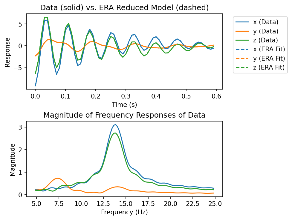
Tweak the range of the FFT plot:
# Tolerance is 0.01
# Automatic mode
# Will not include overdamped modes
# Will create legend for plot
# Will produce FFT plot and limit frequency range to a range of 5 to 25 Hz
fit_era = era.ERA(
    resp_veloc,
    1 / dt,
    svd_tol=0.01,
    auto=True,
    input_labels=['x', 'y', 'z'],
    FFT=True,
    FFT_range=[5, 25],
)
Current fit includes all modes:
  Mode  Freq (Hz)   % Damp    MSV     EMAC   EMACO    MPC     CMIO    MAC
  ----  ---------  --------  ------  ------  ------  ------  ------  ------
*    1     1.3376    1.9494  *0.497  *0.942  *0.943  *0.998  *0.941  *1.000
*    2     7.3891    7.4853  *0.423  *0.986  *0.992  *1.000  *0.992  *1.000
*    3    13.7967    4.9979  *1.000  *0.997  *0.997  *1.000  *0.997  *1.000
Auto-selected modes fit:
  Mode  Freq (Hz)   % Damp    MSV     EMAC   EMACO    MPC     CMIO    MAC
  ----  ---------  --------  ------  ------  ------  ------  ------  ------
     1     1.3376    1.9494   0.497   0.942   0.943   0.998   0.941   1.000
     2     7.3891    7.4853   0.423   0.986   0.992   1.000   0.992   1.000
     3    13.7967    4.9979   1.000   0.997   0.997   1.000   0.997   1.000

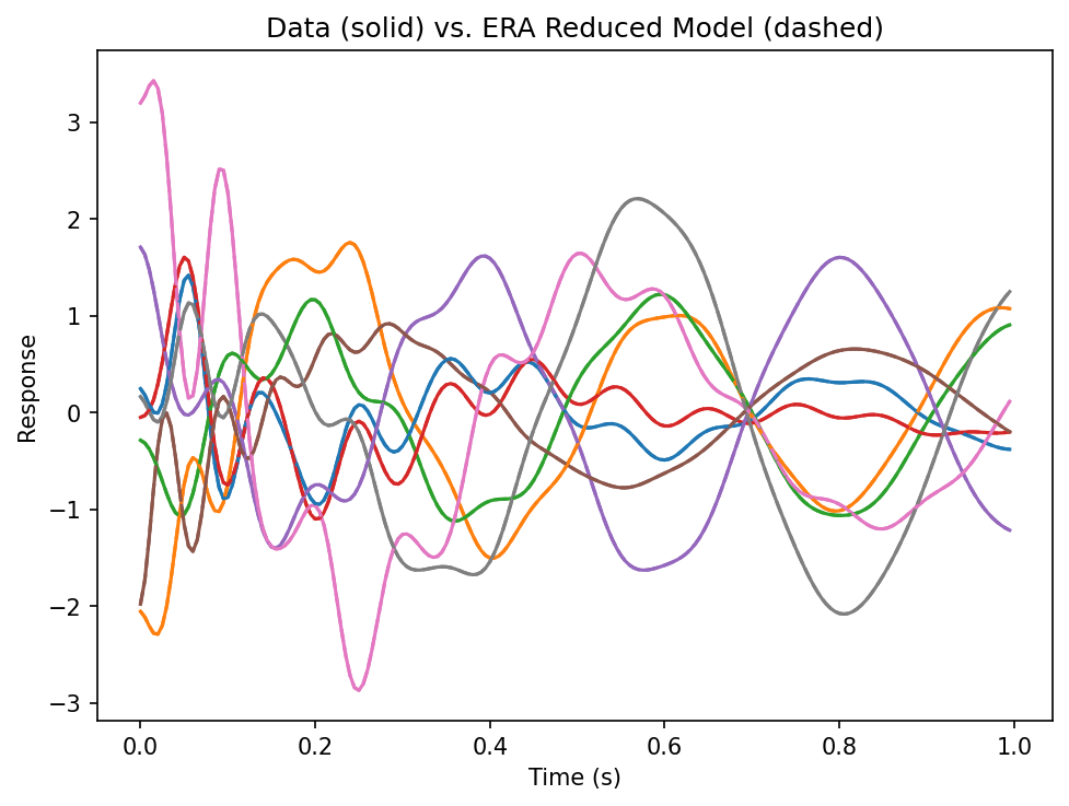
Hands-on Example: A Puzzle
Your task: determine the frequencies and damping of the system that produced the responses given. There is no noise, so your answers should be very precise. Good luck!
To load the data (located here: https://github.com/twmacro/pyyeti/tree/master/docs/tutorials):
from pyyeti import ytools
m = ytools.load("response_data.pgz")
FYI, here is what the response data looks like:

Response Data
# Insert code here
ERA Puzzle Solution
Spoiler alert!
The ‘trick’ to this puzzle is isolating the response data of the system after the impulse input. Looking at the response data (shown above), we can see that there are approximately 0.5 seconds of recorded data before the input, which will not be helpful in identifying any modal contributions to the system. In fact, including this portion of the data will result in a poor ERA fit, or even an error.
# Incorrect solution without trimming the data
m = ytools.load("response_data.pgz")  # Load response data
dt = m['t'][1] - m['t'][0]  # Extract time step

try:
    era_fit = era.ERA(
        m['resp'],  # System response
        1/dt,  # Sample rate
        auto=True,
        MSV_lower_limit=0.5,
    )
except RuntimeError as e:
    print(f"ERA failed:\n{e}")
Current fit includes all modes:
  Mode  Freq (Hz)   % Damp    MSV     EMAC   EMACO    MPC     CMIO    MAC
  ----  ---------  --------  ------  ------  ------  ------  ------  ------
     1     1.4810    3.6212  *0.698  *0.496   0.498   0.384   0.192  *1.000
     2     2.1126    0.7435  *1.000   0.111   0.111   0.029   0.003  *1.000
*    3     2.7416    3.0328  *0.878  *0.538  *0.542  *0.696  *0.377  *1.000
     4     4.1264    9.5263  *0.502   0.000   0.000  *0.879   0.000  *0.993
     5     5.8167    7.0299   0.385   0.000   0.000   0.276   0.000  *0.975
     6     8.1585    6.1471   0.385   0.000   0.000   0.205   0.000  *0.981
     7     9.7788    2.9265  *0.623  *0.376  *0.532  *0.640   0.341  *0.997
     8    10.7540    3.6376  *0.608   0.061   0.232  *0.822   0.191  *0.995
     9    12.3223    3.3606   0.462   0.000   0.002  *0.822   0.002  *0.980
    10    14.0146    2.6025   0.407   0.000   0.000  *0.513   0.000  *0.970
    11    15.5164    1.9179   0.374   0.000   0.177   0.271   0.048  *0.972
    12    16.9043    1.3939   0.281   0.000   0.000   0.188   0.000  *0.934

Auto-selected modes fit:
  Mode  Freq (Hz)   % Damp    MSV     EMAC   EMACO    MPC     CMIO    MAC
  ----  ---------  --------  ------  ------  ------  ------  ------  ------
     1     2.7416    3.0328   1.000   0.538   0.542   0.696   0.377   1.000

If we trim the response data to the relevant system response, our ERA fit significantly improves, and the ERA algorithm can return proper modal data.
print(np.where(m['resp'] == 0)[1][-1]) # This will print the final index at which the system is at rest
99
# Correct solution with data trimming
# From above investigation, we know that the impulse response data starts
# at index 100
dt = m['t'][1] - m['t'][0]  # Extract time step

era_fit = era.ERA(
    m['resp'][:, 100:],  # Trimmed system response after input impulse
    1/dt,  # Sample rate
    auto=True,
    MSV_lower_limit=0.25,  # adjusted lower to keep the 4th mode
)
Current fit includes all modes:
  Mode  Freq (Hz)   % Damp    MSV     EMAC   EMACO    MPC     CMIO    MAC
  ----  ---------  --------  ------  ------  ------  ------  ------  ------
*    1     1.8000    5.0000  *0.967  *1.000  *1.000  *1.000  *1.000  *1.000
*    2     2.5000    2.0000  *1.000  *1.000  *1.000  *1.000  *1.000  *1.000
*    3    10.0000    6.0000  *0.525  *1.000  *1.000  *1.000  *1.000  *1.000
*    4    16.0000   10.0000  *0.285  *1.000  *1.000  *1.000  *1.000  *1.000
Auto-selected modes fit:
  Mode  Freq (Hz)   % Damp    MSV     EMAC   EMACO    MPC     CMIO    MAC
  ----  ---------  --------  ------  ------  ------  ------  ------  ------
     1     1.8000    5.0000   0.967   1.000   1.000   1.000   1.000   1.000
     2     2.5000    2.0000   1.000   1.000   1.000   1.000   1.000   1.000
     3    10.0000    6.0000   0.525   1.000   1.000   1.000   1.000   1.000
     4    16.0000   10.0000   0.285   1.000   1.000   1.000   1.000   1.000

You are encouraged to experiment with keeping/discarding different modes to see their effect on the ERA fit. For example, in this puzzle, the automatic selection of modes while keeping all defaults would give a poor fit since the mode at 16 Hz is discarded due to its low MSV score. When all 4 detected modes are kept, there is an excellent ERA fit and we can clearly see that the frequencies and damping of the system are as follows:
1.8 Hz, 0.05
2.5 Hz, 0.02
10.0 Hz, 0.06
16 Hz, 0.10