pyyeti.era.ERA

class pyyeti.era.ERA(resp, sr, *, svd_tol=0.05, auto=False, alpha=None, beta=None, MSV_lower_limit=0.35, EMAC_lower_limit=0.35, EMACO_lower_limit=0.5, MPC_lower_limit=0.5, CMIO_lower_limit=0.35, MAC_lower_limit=0.75, all_lower_limits=None, damp_range=(0.001, 0.999), freq_range=None, t0=0.0, verbose=True, show_plot=True, input_labels=None, FFT=False, FFT_range=None, figure_label='ERA Fit')

Implements the Eigensystem Realization Algorithm (ERA).

ERA follows minimum realization theory to identify modal parameters (natural frequencies, mode shapes, and damping) from impulse response (free-decay) data. In the absense of forces, the response is completely determined by the system parameters which allows modal parameter identification to work. This code is based on Chapter 5 of reference [1].

The discrete (z-domain) state-space equations are:

x[k+1] = A*x[k] + B*u[k]
y[k]   = C*x[k] + D*u[k]

where u[k] are the inputs, y[k] are the outputs, and x[k] is the state vector at time step k. ERA determines A, B, and C. D is discussed below.

Let there be n_outputs outputs, n_inputs inputs, and n_tsteps time steps. In ERA, impulse response measurements (accelerometer data, for example) form a 3-dimensional matrix sized n_outputs x n_tsteps x n_inputs. This data can be partitioned into n_tsteps n_outputs x n_inputs matrices. These n_outputs x n_inputs matrices are called Markov parameters. ERA computes a set of state-space matrices (A, B, and C) from these Markov parameters. To begin to see a relation between the Markov parameters and the state-space matrices, consider the following. Each input u[k] is assumed to be unity impulse for one DOF and zero elsewhere. For example, if there are two inputs, u0[k] and u1[k], they are assumed to be (for all k):

u0 = [ 1.0, 0.0, 0.0, ... 0.0 ]       # n_inputs x n_tsteps
     [ 0.0, 0.0, 0.0, ... 0.0 ]

u1 = [ 0.0, 0.0, 0.0, ... 0.0 ]       # n_inputs x n_tsteps
     [ 1.0, 0.0, 0.0, ... 0.0 ]

Letting x[0] be zeros (zero initial conditions), iterating through the state-space equations yields these definitions for the outputs:

y0[k] = C @ A ** (k - 1) @ B[:, 0]    # n_outputs x 1

y1[k] = C @ A ** (k - 1) @ B[:, 1]    # n_outputs x 1

Putting these together:

Y[k] = [ y0[k], y1[k] ]                # n_outputs x n_inputs

The Y[k] matrices are the Markov parameters written as a function of the to-be-determined state-space matrices A, B, and C. From the above, it can be seen that D = Y[0]. By equating the input Markov parameters with the expressions for Y[k], ERA computes a minimum realization for A, B, and C.

Note

This is a special note regarding overdamped modes. This algorithm may or may not print the correct frequencies and damping for overdamped modes. Overdamped modes have real eigenvalues, and there is no way for this routine to know which real eigenvalue forms a pair with which other real eigenvalue (see pyyeti.ode.get_freq_damping()). However, the state-space matrices and the fit (see the resp_era attribute) computed by the ERA algorithm will be correct. Note that for underdamped modes, the printed frequency and damping values are correct because this routine sorts the complex eigenvalues to ensure consecutive ordering of these mode pairs.

Note

This routine is demonstrated in the pyYeti Tutorials: Eigensystem Realization Algorithm Tutorial. There is also a link to the source Jupyter notebook at the top of the tutorial.

Mode indicators:

Indicator	Description
MSV	Normalized mode singular value. The MSV value ranges from 0.0 to 1.0 for each mode and is a measure of contribution to the response. Larger values represent larger contribution.
EMAC	Extended modal amplitude coherence. The EMAC value ranges from 0.0 to 1.0 for each mode and is a temporal measure indicating the consistency of the mode over time to the fit. Higher values indicate higher consistency, meaning that the mode decays as expected. The EMAC is computed based on both observability (outputs) and controllability (inputs). From experience, the EMAC is superior to the MAC value (see below). For more information, see [2]. See also EMACO.
EMACO	EMAC from just observability, as opposed to both observability and controllability. Reference [3] argues that this is more reliable than EMAC because there are typically more response measurements (observability side) than inputs (controllability side). This means we are relying on the mode shape matrix C, which is typically supported by many measurements, and not relying on the mode participation factors matrix B, which may be more sensitive to the particular excitation. As pointed out in [3], temporal consistency based on B is highly dependent on the choice of input locations, which may be too few for reliable results. Note Note: this algorithm does not use the equation in [3], which is a simple average of all EMAC values for a mode across all outputs. Instead, it uses a weighted average where the weighting factor for each output is the modeshape coefficient for that output (as done in [2]).
MPC	Modal phase collinearity. The MPC value ranges from 0.0 to 1.0 for each mode and is a spatial measure indicating whether or not the different response locations for a mode are in phase. Higher values indicate more “in-phase” measurements. Only useful if there are multiple outputs (MPC is 1.0 for single output). MPC will be 1.0 for a mode that is 100% real (this happens when the real mode diagonalizes the damping). MPC is directly related to the “Modal Complexity Factor” (MCF): MPC = 1 - MCF.
CMIO	Consistent mode indicator based on observability. CMIO = EMACO * MPC for each mode.
MAC	Modal amplitude coherence. The MAC value ranges from 0.0 to 1.0 for each mode and is a temporal measure indicating the importance of the mode over time to the fit. Higher values indicate more importance. The MAC value for a mode is the dot product of two vectors: The ideal, reconstructed time history for a mode The time history extracted from the input data for the mode after discarding noisy data via singular value decomposition From experience, this indicator is not as useful as the EMAC.

References

[1] (1,2)

Jer-Nan Juang. Applied System Identification. United Kingdom: Prentice Hall, 1994.

[2] (1,2)

Richard S. Pappa, Kenny B. Elliott, Axel Schenk. “A Consistent-Mode Indicator for the Eigensystem Realization Algorithm”, NASA Technical Memorandum 107607, April 1992.

[3] (1,2,3)

Yun, G. J., Lee, S. G., & Shang, S. “An improved mode accuracy indicator for Eigensystem Realization Analysis (ERA) techniques”, KSCE Journal of Civil Engineering, 16, 377-387, March 2012.

Examples

The following example demonstrates ERA by comparing to a known system.

We have the following mass, damping and stiffness matrices (note that the damping has been specially defined to be diagonalized by the modes):

>>> import numpy as np
>>> import scipy.linalg as la
>>> from pyyeti import era, ode
>>> np.set_printoptions(precision=5, suppress=True)
>>>
>>> M = np.identity(3)
>>>
>>> K = np.array(
...     [
...         [4185.1498, 576.6947, 3646.8923],
...         [576.6947, 2104.9252, -28.0450],
...         [3646.8923, -28.0450, 3451.5583],
...     ]
... )
>>>
>>> D = np.array(
...     [
...         [4.96765646, 0.97182432, 4.0162425],
...         [0.97182432, 6.71403672, -0.86138453],
...         [4.0162425, -0.86138453, 4.28850828],
...     ]
... )

Since we have the system matrices, we can determine the frequencies and damping using the eigensolution.

>>> (w2, phi) = la.eigh(K, M)
>>> omega = np.sqrt(w2)
>>> freq_hz = omega / (2 * np.pi)
>>> freq_hz
array([  1.33603,   7.39083,  13.79671])
>>> modal_damping = phi.T @ D @ phi
>>> modal_damping
array([[ 0.33578, -0.     , -0.     ],
       [-0.     ,  6.9657 ,  0.     ],
       [-0.     ,  0.     ,  8.66873]])
>>> zeta = np.diag(modal_damping) / (2 * omega)
>>> zeta
array([ 0.02 ,  0.075,  0.05 ])

What if we only had the response measurements from an impulse input and didn’t have the system matrices? That’s where ERA comes in and we’ll use it to compute modes and damping. Since there is no noise and all modes are excited, ERA will find the exact modes and damping.

First, we need to generate an impulse response for ERA to work with. We’ll just use an initial velocity condition as the source of the impulse:

>>> dt = 0.01
>>> t = np.arange(0, 1, dt)
>>> F = np.zeros((3, len(t)))
>>> ts = ode.SolveUnc(M, D, K, dt)
>>> sol = ts.tsolve(force=F, v0=[1, 1, 1])

We can use the displacement, velocity or acceleration response as the input for ERA. Here, we’ll use velocity because all modes are well represented in the response for the one second simulation. Displacement favors the lower frequency modes (so ERA might eliminate the highest frequency mode) and acceleration favors the higher frequency modes (so ERA might eliminate the lowest frequency mode). For those new to ERA, it is a very good exercise to experiment with using each of them with this problem.

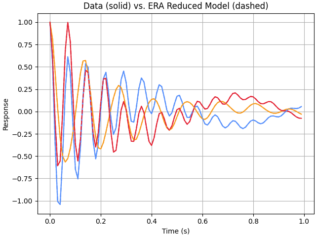
>>> era_fit = era.ERA(
...     sol.v,
...     sr=1 / dt,
...     auto=True,
... )

Current fit includes all modes:
  Mode  Freq (Hz)   % Damp    MSV     EMAC   EMACO    MPC     CMIO    MAC
  ----  ---------  --------  ------  ------  ------  ------  ------  ------
*    1     1.3360    2.0000  *0.817  *1.000  *1.000  *1.000  *1.000  *1.000
*    2     7.3908    7.5000  *0.839  *1.000  *1.000  *1.000  *1.000  *1.000
*    3    13.7967    5.0000  *1.000  *1.000  *1.000  *1.000  *1.000  *1.000

Auto-selected modes fit:
  Mode  Freq (Hz)   % Damp    MSV     EMAC   EMACO    MPC     CMIO    MAC
  ----  ---------  --------  ------  ------  ------  ------  ------  ------
     1     1.3360    2.0000   0.817   1.000   1.000   1.000   1.000   1.000
     2     7.3908    7.5000   0.839   1.000   1.000   1.000   1.000   1.000
     3    13.7967    5.0000   1.000   1.000   1.000   1.000   1.000   1.000

Compare frequencies, damping, mode shapes:

>>> np.allclose(era_fit.freqs_hz, freq_hz)
True
>>> np.allclose(era_fit.zeta, zeta)
True
>>> era_fit.phi / phi  # modes will be scaled differently
array([[ 1.38989, -1.02337, -1.34712],
       [ 1.38989, -1.02337, -1.34712],
       [ 1.38989, -1.02337, -1.34712]])

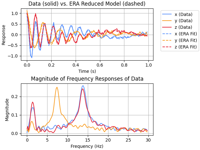
For demonstration, add some noise to the signal and rerun ERA. Note that while this example works out nicely for our known system, it will often be necessary to run ERA multiple times with different parameters and different response data selections to gain confidence in which modes are real.

For this run, we’ll also add some labels and some FFT plots up to 30.0 Hz.

>>> # for repeatability, create a specific generator:
>>> from numpy.random import Generator, PCG64DXSM
>>> rng = Generator(PCG64DXSM(seed=1))
>>> era_fit = era.ERA(
...     sol.v + 0.05 * rng.normal(size=sol.v.shape),
...     sr=1 / dt,
...     auto=True,
...     input_labels=["x", "y", "z"],
...     FFT=True,
...     FFT_range=30.0,
... )

Current fit includes all modes:
  Mode  Freq (Hz)   % Damp    MSV     EMAC   EMACO    MPC     CMIO    MAC
  ----  ---------  --------  ------  ------  ------  ------  ------  ------
*    1     1.3330    6.5080  *0.838  *0.761  *0.779  *0.946  *0.737  *1.000
     2     2.2398   36.5472   0.299   0.010   0.037   0.122   0.005  *0.988
*    3     7.4181    6.9215  *0.851  *0.768  *0.796  *0.999  *0.795  *1.000
     4     8.6995    6.1563   0.267   0.011   0.025  *0.543   0.014  *0.967
*    5    13.7967    4.8219  *1.000  *0.753  *0.837  *0.998  *0.836  *1.000
     6    15.1565    2.0682   0.194   0.013   0.037  *0.794   0.030  *0.930
     7    19.2629    4.0293   0.253   0.007   0.021   0.086   0.002  *0.946
     8    22.1264    1.4390   0.276   0.295   0.408  *0.841   0.343  *0.992
     9    23.6593    9.8029   0.255   0.092   0.277   0.217   0.060  *0.937
    10    28.7943    0.6909   0.178  *0.408  *0.613  *0.910  *0.558  *0.940
    11    32.2365    2.5384   0.211   0.020   0.109   0.482   0.053  *0.952
    12    33.8215    1.7932   0.252   0.063   0.103  *0.843   0.087  *0.978
    13    35.6857    2.1774   0.267   0.057   0.131   0.486   0.064  *0.961
    14    38.6010    1.0741   0.181   0.000   0.000   0.373   0.000  *0.940
    15    42.0391    0.2207   0.191   0.306  *0.500   0.170   0.085  *0.951
    16    45.3651   13.9108   0.066   0.000   0.004  *0.819   0.003   0.286
    17    47.1139    0.5886   0.266   0.278   0.412   0.189   0.078  *0.988

Auto-selected modes fit:
  Mode  Freq (Hz)   % Damp    MSV     EMAC   EMACO    MPC     CMIO    MAC
  ----  ---------  --------  ------  ------  ------  ------  ------  ------
     1     1.3330    6.5080   0.838   0.761   0.779   0.946   0.737   1.000
     2     7.4181    6.9215   0.851   0.768   0.796   0.999   0.795   1.000
     3    13.7967    4.8219   1.000   0.753   0.837   0.998   0.836   1.000

__init__(resp, sr, *, svd_tol=0.05, auto=False, alpha=None, beta=None, MSV_lower_limit=0.35, EMAC_lower_limit=0.35, EMACO_lower_limit=0.5, MPC_lower_limit=0.5, CMIO_lower_limit=0.35, MAC_lower_limit=0.75, all_lower_limits=None, damp_range=(0.001, 0.999), freq_range=None, t0=0.0, verbose=True, show_plot=True, input_labels=None, FFT=False, FFT_range=None, figure_label='ERA Fit')

Instantiates a ERA solver.

Parameters:

• resp (1d, 2d, or 3d ndarray) – Impulse response measurement data. In the general case, this is a 3d array sized n_outputs x n_tsteps x n_inputs, where n_outputs are the number of outputs (measurements), n_tsteps is the number of time steps, and n_inputs is the number of inputs. If there is only one input (the typical case), then resp can be input as a 2d array of size n_outputs x n_tsteps. Further, if there is only one output, then resp can be input as a 1d array of length n_tsteps.

• sr (scalar) – Sample rate at which resp was sampled.

• svd_tol (scalar; optional) –

  Determines how many singular values to keep. Can be:

  • Integer greater than 1 to specify number of expected modes (tolerance equal to 2 * expected modes)

  • Float between 0 and 1 to specify required significance of a singular value to be kept

  Consider this the master control on removal of noise. To change, you have to rerun. When in doubt, it is recommended to try multiple values of svd_tol. The secondary control is the selection of modes which can be interactive (if auto is False) or automatic according to the parameters below.

• auto (boolean; optional) – Enables automatic selection of true modes. The default is False.

• alpha, beta (integers or None; optional) – Number of block rows and block columns to use for the Hankel matrix, respectively. If both are None, the Hankel matrix is made roughly square in terms of blocks. If both are set, alpha is given precedence over beta if there is not enough data to support both settings.

  Note

  The maximum number of modes that can be detected is equal to the minimum dimension of the Hankel matrix divided by 2. So, be careful not to limit either alpha or beta too low.

• MSV_lower_limit (scalar; optional) – The lower limit for the normalized “mode singular value” for modes to be selected when auto is True. The MSV value ranges from 0.0 to 1.0 for each mode.

• EMAC_lower_limit (scalar; optional) – The lower limit for the “extended modal amplitude coherence” value for modes to be selected when auto is True. The EMAC value ranges from 0.0 to 1.0 for each mode.

• EMACO_lower_limit (scalar; optional) – The lower limit for the “extended modal amplitude coherence from observability” value for modes to be selected when auto is True. The EMACO value ranges from 0.0 to 1.0 for each mode.

• MPC_lower_limit (scalar; optional) – The lower limit for the “modal phase collinearity” value for modes to be selected when auto is True. The MPC value ranges from 0.0 to 1.0 for each mode.

• CMIO_lower_limit (scalar; optional) – The lower limit for the “consistent mode indicator from observability” value for modes to be selected when auto is True. The CMIO value ranges from 0.0 to 1.0 for each mode.

• MAC_lower_limit (scalar; optional) – The lower limit for the “modal amplitude coherence” value for modes to be selected when auto is True. The MAC value ranges from 0.0 to 1.0 for each mode.

• all_lower_limits (scalar or None; optional) – If not None, it sets all the indicator lower limit values and any other lower limit settings are quietly ignored.

• damp_range (2-tuple; optional) – Specifies the range (inclusive) of acceptable damping values for automatic selection.

• freq_range (2-tuple or None; optional) – Specifies the range (inclusive) of acceptable frequencies (in Hz) values for automatic selection. If None (the default), freq_range = (0, sr/2).

• t0 (scalar; optional) – The initial time value in resp. Only used for plotting.

• verbose (bool; optional) – If True, print tables showing frequencies and indicators. Ignored (treated as True) if auto is False.

• show_plot (boolean; optional) – If True, show plot of ERA fit (with or without FFT). The default is True.

• input_labels (list or None; optional) – List of data labels for each input signal to ERA.

• FFT (boolean; optional) – Enables display of FFT plot of input data. The default is False.

• FFT_range (scalar or list; optional) – Limits displayed frequency range of FFT plot. A scalar value or list with one term will act as a maximum cutoff. A pair of values will act as minimum and maximum cutoffs, respectively. The default is None.

• figure_label (string; optional) – Label to use for opening figures. Handy for comparing different ERA fits side-by-side.

Notes

The class instance is populated with the following members (equation numbers are from Chapter 5 of reference [1]):

Member	Description
resp	Impulse response data
resp_era	Final ERA fit to the impulse response data
n_outputs	Number of outputs
n_tsteps	Number of time-steps
n_inputs	Number of inputs
sr	Sample rate
t0	Initial time value in resp (for plotting)
time	resp time vector used for plotting; created from sr and t0
svd_tol	Singular value tolerance
auto	Automatic or interactive method of identifying true modes
show_plot	If True, plots are made
input_labels	Create a legend for approximated fit plot
lower_limits	Dict of lower limits for each indicator for auto-selecting modes
damp_range	Range of acceptable damping values for automatic selection
freq_range	Range of acceptable frequencies (Hz) for automatic selection
FFT	Produces an FFT plot of input data for comparison to detected modes
FFT_range	Frequency cutoff(s) for FFT plot
figure_label	Label for figure windows
H_0	The H(0) generalized Hankel matrix (eq 5.24)
H_1	The H(1) generalized Hankel matrix (eq 5.24)
alpha	Number of block rows (time-steps) in H
beta	Number of block columns (time-steps) in H
A_hat	ERA state-space “A” matrix, (eq 5.34)
B_hat	ERA state-space “B” matrix, (eq 5.34)
C_hat	ERA state-space “C” matrix, (eq 5.34)
A_modal	ERA modal state-space “A” matrix (complex eigenvalues on diagonal)
B_modal	ERA modal state-space “B” matrix
C_modal	ERA modal state-space “C” matrix (complex mode-shapes)
eigs	Complex eigenvalues of A_hat (discrete)
eigs_continuous	Continuous version of eigs; ln(eigs) * sr
psi	Complex eigenvectors of A_hat
psi_inv	Inverse of psi
freqs	Real mode frequencies (rad/sec)
freqs_hz	Real mode frequencies (Hz)
zeta	Real mode percent critical damping
phi	Real mode shapes (from C_modal); see also the MPC results for how “real” each mode is
indicators	Dict of all indicator values for each mode pair

Methods

__init__(resp, sr, *[, svd_tol, auto, ...])

Instantiates a ERA solver.