Checking data recovery matrices: modal DOF (cb.cbtf)
This and other notebooks are available here: https://github.com/twmacro/pyyeti/tree/master/docs/tutorials.
As with the cbcheck tutorial, we’ll use superelement 102. The data recovery matrices were formed in the test directory: “tests/nastran_drm12”.
The cbtf routine aides in checking the modal DOF. This function performs a base-drive analysis and returns the boundary and modal responses. These are then used by the analyst to plot frequency response curves as a sanity check.
Notes:
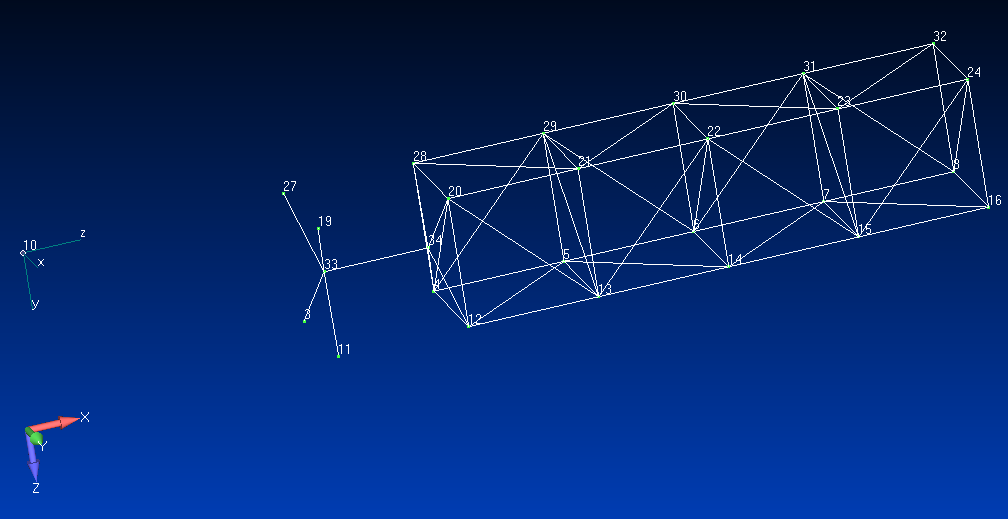
This model uses units of kg, mm, s
It’s a very light-weight truss: mass = 1.755 kg
First, do some imports:
import numpy as np
import matplotlib.pyplot as plt
from pyyeti import cb, nastran
np.set_printoptions(precision=3, linewidth=130, suppress=True)
Some settings specifically for the jupyter notebook.
%matplotlib inline
plt.rcParams['figure.figsize'] = [6.4, 4.8]
plt.rcParams['figure.dpi'] = 150.
Need path to data files:
import os
import inspect
pth = os.path.dirname(inspect.getfile(cb))
pth = os.path.join(pth, 'tests', 'nastran_drm12')
Load data recovery matrices
We’ll use the function
procdrm12
from the nastran.op2 module. (This
gets imported into the nastran namespace automatically.)
otm = nastran.procdrm12(os.path.join(pth, 'drm12'))
Processing "Displacement" requests...
Processing "Acceleration" requests...
Processing "SPC Force" requests...
Processing "Stress" requests...
Processing "Element Force" requests...
sorted(otm.keys())
['ATM',
 'ATM_desc',
 'ATM_id_dof',
 'DTMA',
 'DTMD',
 'DTM_desc',
 'DTM_id_dof',
 'LTMA',
 'LTMD',
 'LTM_desc',
 'LTM_id_dof',
 'SPCFA',
 'SPCFD',
 'SPCF_desc',
 'SPCF_id_dof',
 'STMA',
 'STMD',
 'STM_desc',
 'STM_id_dof']
Load the mass and stiffness from the “nas2cam” output
Use the op2.rdnas2cam routine (imported from nastran.op2) to read data from the output of the “nas2cam” DMAP. This loads the data into a dict:
nas = nastran.rdnas2cam(os.path.join(pth, 'inboard_nas2cam'))
nas.keys()
dict_keys(['uset', 'cstm', 'cstm2', 'maps', 'dnids', 'upids', 'selist', 'lambda', 'maa', 'kaa'])
maa = nas['maa'][102]
kaa = nas['kaa'][102]
Get the USET table for the b-set DOF
uset = nas['uset'][102]
b = nastran.mksetpv(uset, 'p', 'b')
usetb = uset[b]
# show the coordinates (which are in basic):
usetb.loc[(slice(None), 1), :]
| nasset | x | y | z | ||
|---|---|---|---|---|---|
| id | dof | ||||
| 3 | 1 | 2 | 600.0 | 0.0 | 300.0 |
| 11 | 1 | 2 | 600.0 | 300.0 | 300.0 |
| 19 | 1 | 2 | 600.0 | 300.0 | 0.0 |
| 27 | 1 | 2 | 600.0 | 0.0 | 0.0 |
Form b-set partition vector into a-set
In this case, we already know the b-set are first but, since we have the nas2cam output, we can use n2p.mksetpv to be more general. We’ll also get the q-set partition vector for later use.
b = nastran.mksetpv(uset, 'a', 'b')
q = ~b
b = np.nonzero(b)[0]
q = np.nonzero(q)[0]
print('b =', b)
print('q =', q)
b = [ 0  1  2  3  4  5  6  7  8  9 10 11 12 13 14 15 16 17 18 19 20 21 22 23]
q = [24 25 26 27 28 29 30 31 32 33 34 35 36 37 38 39 40 41 42 43 44 45 46 47 48 49 50 51 52 53 54 55 56 57 58 59 60 61 62 63 64 65 66
 67 68 69 70 71 72 73 74 75 76 77 78 79 80 81 82 83]
Form the damping matrix
We’ll use 2.5% critical damping.
baa = 2*.025*np.sqrt(np.diag(kaa))
baa[b] = 0
baa = np.diag(baa)
Form rigid-body modes
These are used to define the acceleration(s) of the boundary DOF. Each rigid-body mode defines a consistent acceleration field which is needed for a base-drive (which is really what cbtf does).
Note the the second boundary grid is in a different coordinate system.
rbg = nastran.rbgeom_uset(usetb, [600, 150, 150])
rbg
array([[   1.,    0.,    0.,    0.,  150.,  150.],
       [   0.,    1.,    0., -150.,    0.,    0.],
       [   0.,    0.,    1., -150.,    0.,    0.],
       [   0.,    0.,    0.,    1.,    0.,    0.],
       [   0.,    0.,    0.,    0.,    1.,    0.],
       [   0.,    0.,    0.,    0.,    0.,    1.],
       [   0.,    1.,    0., -150.,    0.,    0.],
       [   0.,    0.,    1.,  150.,    0.,    0.],
       [   1.,    0.,    0.,    0.,  150., -150.],
       [   0.,    0.,    0.,    0.,    1.,    0.],
       [   0.,    0.,    0.,    0.,    0.,    1.],
       [   0.,    0.,    0.,    1.,    0.,    0.],
       [   1.,    0.,    0.,    0., -150., -150.],
       [   0.,    1.,    0.,  150.,    0.,    0.],
       [   0.,    0.,    1.,  150.,    0.,    0.],
       [   0.,    0.,    0.,    1.,    0.,    0.],
       [   0.,    0.,    0.,    0.,    1.,    0.],
       [   0.,    0.,    0.,    0.,    0.,    1.],
       [   1.,    0.,    0.,    0., -150.,  150.],
       [   0.,    1.,    0.,  150.,    0.,    0.],
       [   0.,    0.,    1., -150.,    0.,    0.],
       [   0.,    0.,    0.,    1.,    0.,    0.],
       [   0.,    0.,    0.,    0.,    1.,    0.],
       [   0.,    0.,    0.,    0.,    0.,    1.]])
Do a check of the mass:
bb = np.ix_(b, b)
rbg.T @ maa[bb] @ rbg
array([[      1.755,       0.   ,      -0.   ,       0.   ,       0.   ,       0.   ],
       [      0.   ,       1.755,      -0.   ,      -0.   ,       0.   ,     772.22 ],
       [     -0.   ,      -0.   ,       1.755,       0.   ,    -772.22 ,      -0.   ],
       [      0.   ,      -0.   ,       0.   ,   35905.202,      -0.   ,      -0.   ],
       [      0.   ,       0.   ,    -772.22 ,      -0.   ,  707976.725,     109.558],
       [      0.   ,     772.22 ,      -0.   ,      -0.   ,     109.558,  707976.725]])
Define analysis frequency vector and run cbtf
The save option is useful for speeding up loops 2 to 6:
freq = np.arange(0.1, 200., .1)
save = {}
sol = {}
for i in range(6):
    sol[i] = cb.cbtf(maa, baa, kaa, rbg[:, i], freq, b, save)
Each solution (eg, sol[0]) has:
The boundary and modal accelerations, velocities and displacements (
.a, .v, .d)The boundary force (
.frc)The analysis frequency vector (
.freq)
[i for i in dir(sol[0]) if i[0] != '_']
['a', 'd', 'f', 'frc', 'freq', 'v']
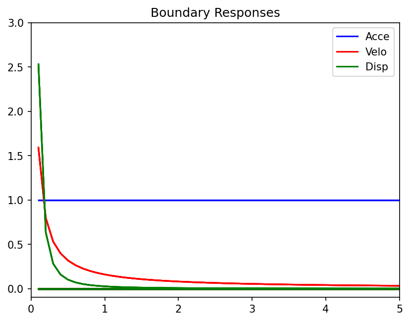
Just to check the solution, we’ll first look at the boundary responses. The acceleration should be the same as the input (0 or 1), and velocity & displacement should be large approaching zero, but approach zero as frequency increases. (They should equal 1 where \(2\pi f\) is 1, or \(f \approx 0.16\).) Off-axis values should be zero.
h = plt.plot(freq, abs(sol[0].a[b]).T, 'b',
             freq, abs(sol[0].v[b]).T, 'r',
             freq, abs(sol[0].d[b]).T, 'g')
plt.title('Boundary Responses')
plt.legend(h[::len(b)], ('Acce', 'Velo', 'Disp'), loc='best')
plt.ylim(-.1, 3)
plt.xlim(0, 5)
(0.0, 5.0)
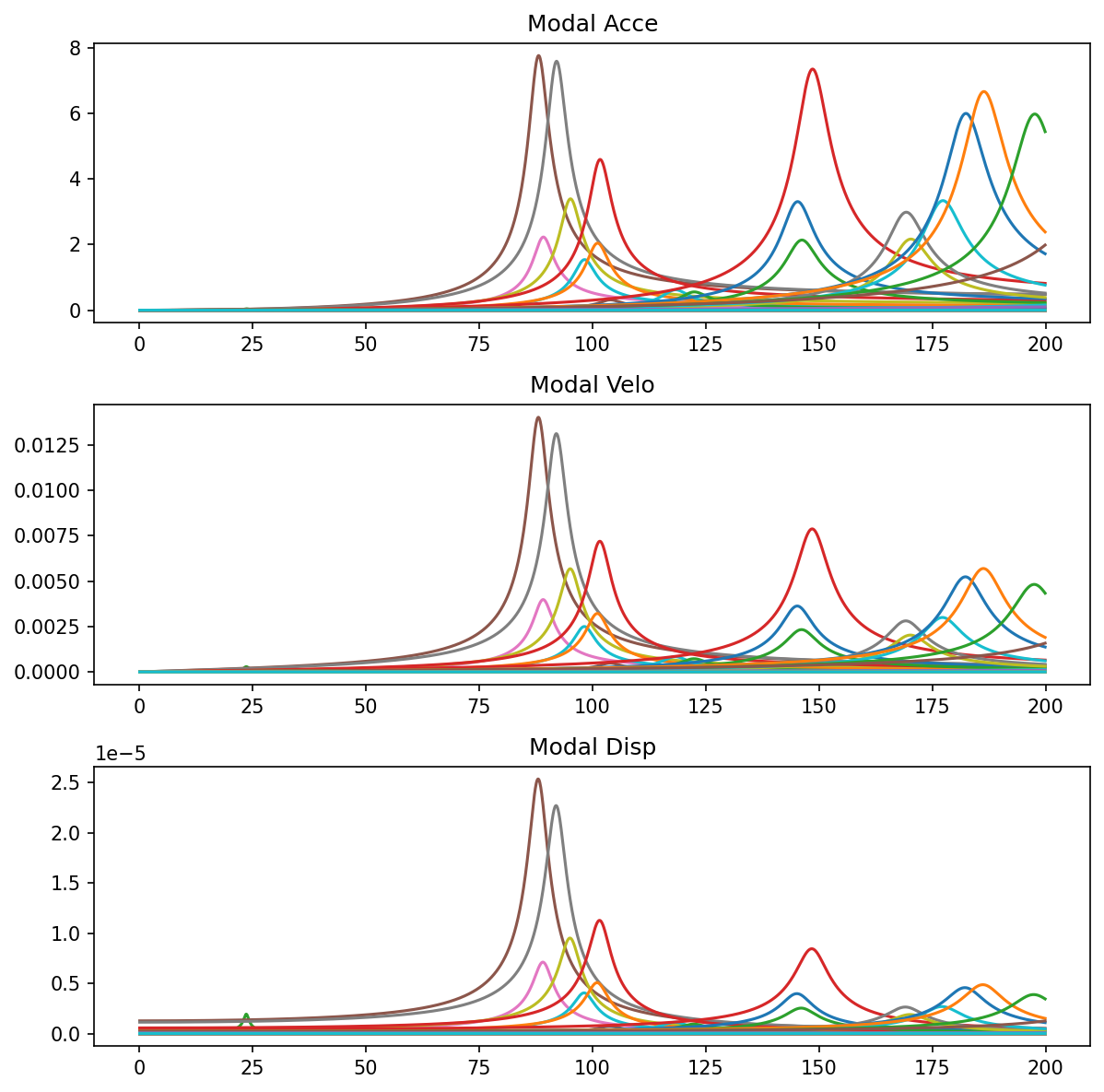
The modal part has dynamic content as we’ll see next. Note: for the x-direction, the modes of interest are above 50 Hz. The other directions have modal content much lower in frequency.
plt.figure(figsize=(8, 8))
plt.subplot(311); plt.plot(freq, abs(sol[0].a[q]).T); plt.title('Modal Acce')
plt.subplot(312); plt.plot(freq, abs(sol[0].v[q]).T); plt.title('Modal Velo')
plt.subplot(313); plt.plot(freq, abs(sol[0].d[q]).T); plt.title('Modal Disp')
plt.tight_layout()
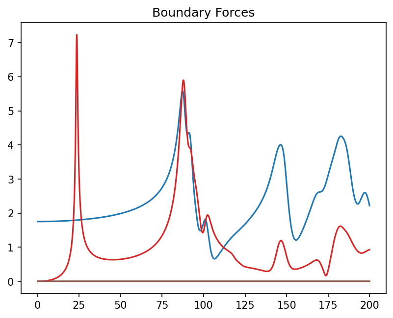
We can plot sol.frc to see the boundary forces needed to run the
base-drive. Here, we’ll use the rigid-body modes to sum the forces to
the center point and plot that. The starting value for the x-direction
should be 1.755 to match the mass.
plt.plot(freq, abs(rbg.T @ sol[0].frc).T)
plt.title('Boundary Forces');
Finally, let’s get to checking the data recovery matrices.
The first one we’ll check is the SPCF recovery. Since that was
defined to recovery the boundary forces, the components should match the
b-set parts of the mass and stiffness. (Note that SPCFD loses some
precision through the DMAP as compared to the original stiffness.)
assert np.allclose(otm['SPCFA'], maa[b])
assert np.allclose(otm['SPCFD'], kaa[bb])
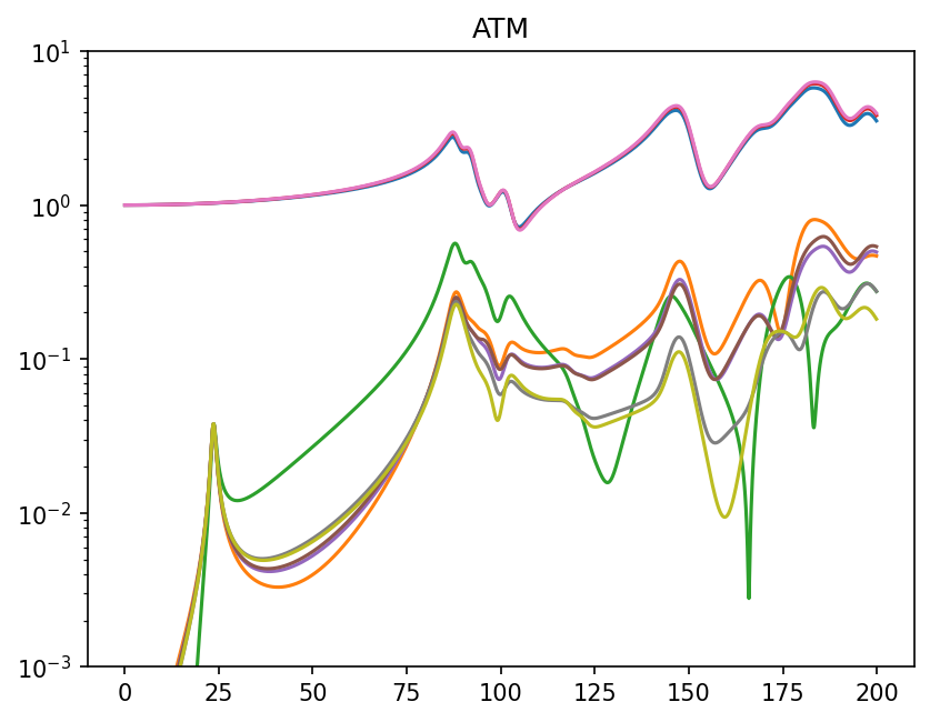
For the ATM, there should be some lines that start at 1.0. Other
lines, should start at zero. These curves make sense.
plt.semilogy(freq, abs(otm['ATM'] @ sol[0].a).T)
plt.title('ATM')
plt.ylim(.001, 10)
(0.001, 10)
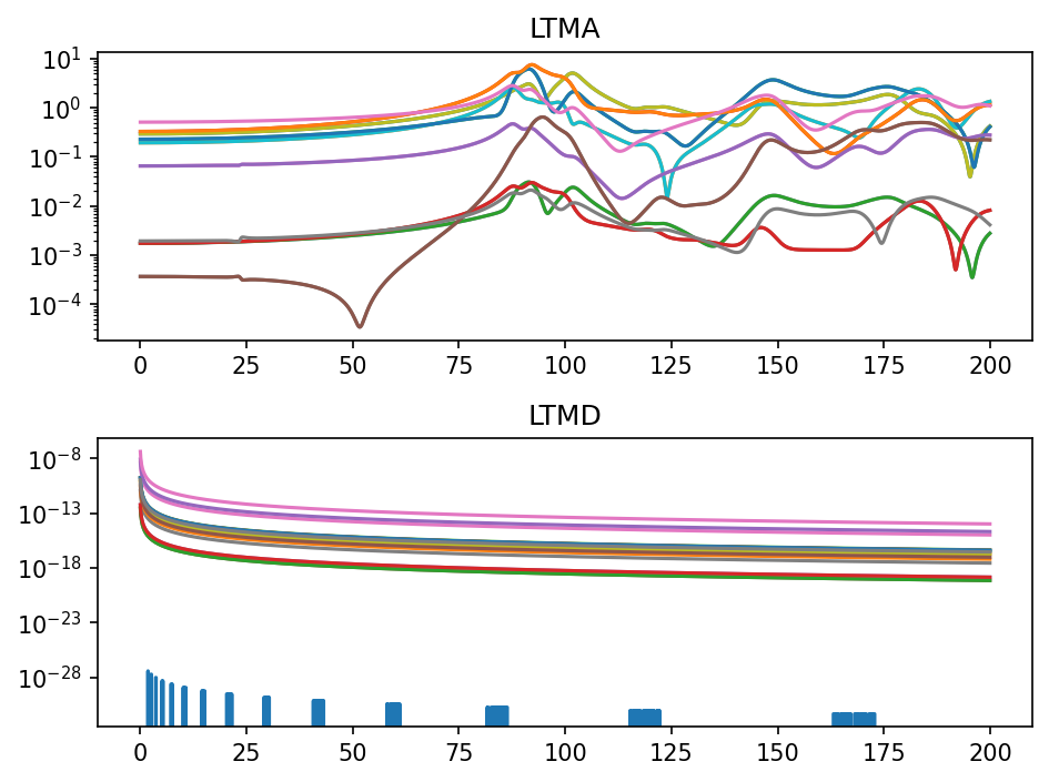
The LTMA curves should all start with zero slope. LTMD curves
should be numerically zero since rigid-body displacement should not
cause any loads. These look reasonable.
plt.subplot(211)
plt.semilogy(freq, abs(otm['LTMA'] @ sol[0].a).T)
plt.title('LTMA')
plt.subplot(212)
plt.semilogy(freq, abs(otm['LTMD'] @ sol[0].d[b]).T)
plt.title('LTMD')
plt.tight_layout()
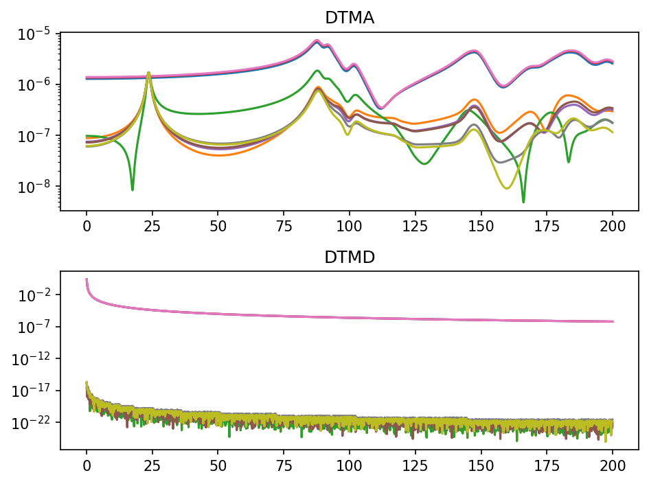
The DTMA curves should also start with zero slope, with values much
less than 1.0. Some of the DTMD curves (the ones in the ‘x’
direction) should start at high values then quickly drop off as
frequency increases.
plt.subplot(211)
plt.semilogy(freq, abs(otm['DTMA'] @ sol[0].a).T)
plt.title('DTMA')
plt.subplot(212)
plt.semilogy(freq, abs(otm['DTMD'] @ sol[0].d[b]).T)
plt.title('DTMD')
plt.tight_layout()