pyyeti.ode.SolveExp1
- class pyyeti.ode.SolveExp1(A, h, order=1)[source]
1st order ODE time domain solver based on the matrix exponential.
This class is for solving:
yd - A y = fThis solver is exact assuming either piece-wise linear or piece-wise constant forces. See
SolveExp2for more details on how this algorithm solves the ODE.Examples
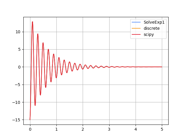
Calculate impulse response of state-space system:
xd = A @ x + B @ u
y  = C @ x + D @ u
- where:
force = 0’s
velocity(0) = B
>>> from pyyeti import ode
>>> from pyyeti.ssmodel import SSModel
>>> import numpy as np
>>> import matplotlib.pyplot as plt
>>> f = 5           # 5 hz oscillator
>>> w = 2*np.pi*f
>>> w2 = w*w
>>> zeta = .05
>>> h = .01
>>> nt = 500
>>> A = np.array([[0, 1], [-w2, -2*w*zeta]])
>>> B = np.array([[0], [3]])
>>> C = np.array([[8, -5]])
>>> D = np.array([[0]])
>>> F = np.zeros((1, nt), float)
>>> ts = ode.SolveExp1(A, h)
>>> sol = ts.tsolve(B @ F, B[:, 0])
>>> y = C @ sol.d
>>> fig = plt.figure('Example')
>>> fig.clf()
>>> ax = plt.plot(sol.t, y.T,
...               label='SolveExp1')
>>> ssmodel = SSModel(A, B, C, D)
>>> z = ssmodel.c2d(h=h, method='zoh')
>>> x = np.zeros((A.shape[1], nt+1), float)
>>> y2 = np.zeros((C.shape[0], nt), float)
>>> x[:, 0:1] = B
>>> for k in range(nt):
...     x[:, k+1] = z.A @ x[:, k] + z.B @ F[:, k]
...     y2[:, k]  = z.C @ x[:, k] + z.D @ F[:, k]
>>> ax = plt.plot(sol.t, y2.T, label='discrete')
>>> leg = plt.legend(loc='best')
>>> np.allclose(y, y2)
True
Compare against scipy:
>>> from scipy import signal
>>> ss = ssmodel.getlti()
>>> tout, yout = ss.impulse(T=sol.t)
>>> ax = plt.plot(tout, yout, label='scipy')
>>> leg = plt.legend(loc='best')
>>> np.allclose(yout, y.ravel())
True
- __init__(A, h, order=1)[source]
Instantiates a
SolveExp1solver.- Parameters:
A (2d ndarray) – The state-space matrix:
yd - A y = fh (scalar or None) – Time step or None; if None, the E, P, Q members will not be computed.
order (scalar, optional) – Specify which solver to use:
0 for the zero order hold (force stays constant across time step)
1 for the 1st order hold (force can vary linearly across time step)
Notes
The class instance is populated with the following members:
Member
Description
A
the input A
h
time step
n
number of total DOF (
A.shape[0])order
order of solver (0 or 1; see above)
E, P, Q
output of
pyyeti.expmint.getEPQ(); they are matrices used to solve the ODEpc
True if E, P, and Q member have been calculated; False otherwise
The E, P, and Q entries are used to solve the ODE:
for j in range(1, nt):
    d[:, j] = E*d[:, j-1] + P*F[:, j-1] + Q*F[:, j]
Methods
__init__(A, h[, order])Instantiates a
SolveExp1solver.tsolve(force[, d0])Solve time-domain 1st order ODE equations.