pyyeti.ode.SolveExp2
- class pyyeti.ode.SolveExp2(m, b, k, h, rb=None, rf=None, order=1, pre_eig=False)[source]
2nd order ODE time domain solver based on the matrix exponential.
This class is for solving matrix equations of motion:
\[M \ddot{q} + B \dot{q} + K q = F\]The 2nd order ODE set of equations are transformed into the 1st order ODE:
\[\begin{split}\left\{ \begin{array}{c} \ddot{q} \\ \dot{q} \end{array} \right\} - \left[ \begin{array}{cc} -M^{-1} B & -M^{-1} K \\ I & 0 \end{array} \right] \left\{ \begin{array}{c} \dot{q} \\ q \end{array} \right\} = \left\{ \begin{array}{c} M^{-1} F \\ 0 \end{array} \right\}\end{split}\]or:
\[\dot{y} - A y = w\]The general solution is:
\[y = e^{A t} \left ( y(0) + \int_0^t {e^{-A \tau} w d\tau} \right )\]By only requiring the solution at every time step and assuming a constant step size of h:
\[y_{n+1} = e^{A h} \left ( y_{n} + \int_0^h {e^{-A \tau} w(t_n+\tau) d\tau} \right )\]By assuming \(w(t_n+\tau)\) is piece-wise linear (if order is 1) or piece-wise constant (if order is 0) for each step, an exact, closed form solution can be calculated. The function
pyyeti.expmint.getEPQ()computes the matrix exponential \(E = e^{A h}\), and solves the integral(s) needed to compute P and Q so that a solution can be computed by:\[y_{n+1} = E y_{n} + P w_{n} + Q w_{n+1}\]Unlike for the uncoupled solver
SolveUnc, this solver doesn’t need or use the rb input unless static initial conditions are requested when solving equations.Note that
SolveUncis also an exact solver assuming piece-wise linear or piece-wise constant forces.SolveUncis often faster thanSolveExp2since it uncouples the equations and therefore doesn’t need to work with matrices in the inner loop. However, it is recommended to experiment with both solvers for any particular application.Note
The above equations are for the non-residual-flexibility modes. The ‘rf’ modes are solved statically and any initial conditions are ignored for them.
For a static solution:
rigid-body displacements = zeros
elastic displacments = inv(k[elastic]) * F[elastic]
velocity = zeros
rigid-body accelerations = inv(m[rigid]) * F[rigid]
elastic accelerations = zeros
See also
Examples
>>> from pyyeti import ode
>>> import numpy as np
>>> m = np.array([10., 30., 30., 30.])    # diag mass
>>> k = np.array([0., 6.e5, 6.e5, 6.e5])  # diag stiffness
>>> zeta = np.array([0., .05, 1., 2.])    # percent damp
>>> b = 2.*zeta*np.sqrt(k/m)*m            # diag damping
>>> h = 0.001                             # time step
>>> t = np.arange(0, .3001, h)            # time vector
>>> c = 2*np.pi
>>> f = np.vstack((3*(1-np.cos(c*2*t)),
...                4.5*(np.cos(np.sqrt(k[1]/m[1])*t)),
...                4.5*(np.cos(np.sqrt(k[2]/m[2])*t)),
...                4.5*(np.cos(np.sqrt(k[3]/m[3])*t))))
>>> f *= 1.e4
>>> ts = ode.SolveExp2(m, b, k, h)
>>> sol = ts.tsolve(f, static_ic=1)
Solve with scipy.signal.lsim for comparison:
>>> A = ode.make_A(m, b, k)
>>> n = len(m)
>>> Z = np.zeros((n, n), float)
>>> B = np.vstack((np.eye(n), Z))
>>> C = np.vstack((A, np.hstack((Z, np.eye(n)))))
>>> D = np.vstack((B, Z))
>>> ic = np.hstack((sol.v[:, 0], sol.d[:, 0]))
>>> import scipy.signal
>>> f2 = (1./m).reshape(-1, 1) * f
>>> tl, yl, xl = scipy.signal.lsim((A, B, C, D), f2.T, t,
...                                X0=ic)
>>> print('acce cmp:', np.allclose(yl[:, :n], sol.a.T))
acce cmp: True
>>> print('velo cmp:', np.allclose(yl[:, n:2*n], sol.v.T))
velo cmp: True
>>> print('disp cmp:', np.allclose(yl[:, 2*n:], sol.d.T))
disp cmp: True
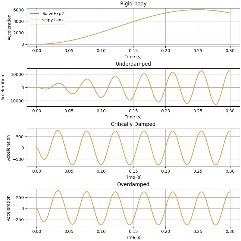
Plot the four accelerations:
>>> import matplotlib.pyplot as plt
>>> fig = plt.figure('Example', figsize=[8, 8], clear=True,
...                  layout='constrained')
>>> labels = ['Rigid-body', 'Underdamped',
...           'Critically Damped', 'Overdamped']
>>> for j, name in zip(range(4), labels):
...     _ = plt.subplot(4, 1, j+1)
...     _ = plt.plot(t, sol.a[j], label='SolveExp2')
...     _ = plt.plot(tl, yl[:, j], label='scipy lsim')
...     _ = plt.title(name)
...     _ = plt.ylabel('Acceleration')
...     _ = plt.xlabel('Time (s)')
...     if j == 0:
...         _ = plt.legend(loc='best')
- __init__(m, b, k, h, rb=None, rf=None, order=1, pre_eig=False)[source]
Instantiates a
SolveExp2solver.- Parameters:
m (1d or 2d ndarray or None) – Mass; vector (of diagonal), or full; if None, mass is assumed identity
b (1d or 2d ndarray) – Damping; vector (of diagonal), or full
k (1d or 2d ndarray) – Stiffness; vector (of diagonal), or full
h (scalar or None) – Time step; can be None if only want to solve a static problem
rb (1d array or None; optional) – Index or bool partition vector for rigid-body modes. Set to [] to specify no rigid-body modes. If None, the rigid-body modes will be automatically detected by this logic for uncoupled systems:
rb = np.nonzero(abs(k).max(0) < 0.005)[0]
And by this logic for coupled systems:
rb = ((abs(k).max(axis=0) < 0.005) &
      (abs(k).max(axis=1) < 0.005) &
      (abs(b).max(axis=0) < 0.005) &
      (abs(b).max(axis=1) < 0.005)).nonzero()[0]
Note
rb applies only to modal-space equations. Use pre_eig if necessary to convert to modal-space. This means that if rb is an index vector, it specifies the rigid-body modes after the pre_eig operation. See also pre_eig.
Note
Unlike for the
SolveUncsolver, rb for this solver is only used if using static initial conditions inSolveExp2.tsolve().rf (1d array or None; optional) – Index or bool partition vector for residual-flexibility modes; these will be solved statically. As for the rb option, the rf option only applies to modal space equations (possibly after the pre_eig operation).
order (integer; optional) – Specify which solver to use:
0 for the zero order hold (force stays constant across time step)
1 for the 1st order hold (force can vary linearly across time step)
pre_eig (bool; optional) – If True, an eigensolution will be computed with the mass and stiffness matrices to convert the system to modal space. This will allow the automatic detection of rigid-body modes which is necessary for specifying “static” initial conditions when calling the solver. No modes are truncated. Only works if stiffness is symmetric/hermitian and mass is positive definite (see
scipy.linalg.eigh()). Just leave it as False if the equations are already in modal space or if not using “static” initial conditions.
Notes
The instance is populated with the following members:
Member
Description
m
mass for the non-rf modes
b
damping for the non-rf modes
k
stiffness for the non-rf modes
m_orig
original mass
b_orig
original damping
k_orig
original stiffness
h
time step
rb
index vector or slice for the rb modes
el
index vector or slice for the el modes
rf
index vector or slice for the rf modes
_rb
index vector or slice for the rb modes relative to the non-rf modes
_el
index vector or slice for the el modes relative to the non-rf modes
nonrf
index vector or slice for the non-rf modes
kdof
index vector or slice for the non-rf modes
n
number of total DOF
rbsize
number of rb modes
elsize
number of el modes
rfsize
number of rf modes
nonrfsz
number of non-rf modes
ksize
number of non-rf modes
invm
decomposition of m for the non-rf, non-rb modes
krf
stiffness for the rf modes
ikrf
inverse of stiffness for the rf modes
unc
True if there are no off-diagonal terms in any matrix; False otherwise
order
order of solver (0 or 1; see above)
E_vv
partition of “E” which is output of
pyyeti.expmint.getEPQ()E_vd
another partition of “E”
E_dv
another partition of “E”
E_dd
another partition of “E”
P, Q
output of
pyyeti.expmint.getEPQ(); they are matrices used to solve the ODEpc
True if E*, P, and Q member have been calculated; False otherwise
pre_eig
True if the “pre” eigensolution was done; False otherwise
phi
the mode shape matrix from the “pre” eigensolution; only present if pre_eig is True
The E, P, and Q entries are used to solve the ODE:
for j in range(1, nt):
    d[:, j] = E*d[:, j-1] + P*F[:, j-1] + Q*F[:, j]
Methods
__init__(m, b, k, h[, rb, rf, order, pre_eig])Instantiates a
SolveExp2solver.finalize([get_force])Finalize time-domain generator solution.
fsolve()'Abstract' method to solve frequency-domain equations
generator(nt, F0[, d0, v0, static_ic])Python "generator" version of
SolveExp2.tsolve(); interactively solve (or re-solve) one step at a time.get_f2x(phi[, velo])Get force-to-displacement or force-to-velocity transform
tsolve(force[, d0, v0, static_ic])Solve time-domain 2nd order ODE equations