pyyeti.ode.SolveUnc
- class pyyeti.ode.SolveUnc(m, b, k, h=None, rb=None, rf=None, order=1, pre_eig=False, cd_as_force=False)[source]
2nd order ODE time and frequency domain solvers for “uncoupled” equations of motion
This class is for solving:
\[M \ddot{q} + C \dot{q} + K q = P\]Note that the mass, damping and stiffness can be fully populated (coupled). If mass and stiffness are diagonal, but damping is coupled, see also
SolveCDF.Like
SolveExp2, this solver is exact assuming piece-wise linear forces (if order is 1) or piece-wise constant forces (if order is 0).Uncoupled Equations
For uncoupled equations, pre-formulated integration coefficients are used as shown in the following displacement and velocity recurrence relations (think of the coefficients as diagonal matrices):
\[ \begin{align}\begin{aligned}\begin{aligned} q_{i+1} &= F q_i + G \dot{q}_i + A P_i + B P_{i+1}\\\dot{q}_{i+1} &= F_p q_i + G_p \dot{q}_i + A_p P_i + B_p P_{i+1} \end{aligned}\end{aligned}\end{align} \]Those coefficients (computed in
get_su_coef()for underdamped, critically-damped, and overdamped systems) can be derived as follows. Consider the equation of motion for a single degree of freedom:\[\ddot{q}(t) + 2 \zeta \omega_n \dot{q}(t) + {\omega_n}^2 q(t) = \frac{1}{m} P(t)\]For illustration, we’ll assume that we have an underdamped system (\(\zeta < 1\)). The exact solution consists of a free-decay part (the homogeneous solution) and a forced-response part (the particular solution):
\[q(t) = e^{-\zeta \omega_n t} \left [ q_0 \cos(\omega_d t) + \frac{v_0 + \zeta \omega_n q_0}{\omega_d} \sin(\omega_d t) \right ] + \frac{1}{m \omega_d} \int_0^t {e^{-\zeta \omega_n (t - \tau)} \sin(\omega_d (t - \tau)) P(\tau) d \tau}\]where the displacement and velocity initial conditions are \(q_0\) and \(v_0\), and \(\omega_d\) is the damped natural frequency:
\[\omega_d = \omega_n \sqrt{1-\zeta^2}\]Consider a single time step, from \(t_n\) to \(t_{n+1}\). If we assume that the force varies linearly within that time step, we can solve the integral in the above equation (Duhamel’s integral) that will be valid from \(t_n\) to \(t_{n+1}\) (\(\tau\) will still range from \(0\) to \(t\)). Given the initial conditions \(q_n\) and \(v_n\) for the time step, we would then have the solution \(q(t)\) that would be valid from \(t_n\) to \(t_{n+1}\). Define the time step size as \(h\). Therefore:
In the equation above, \(t = 0\) now represents \(t_n\) and \(t=h\) represents \(t_{n+1}\)
\(q_0\) becomes \(q_n\) and \(v_0\) becomes \(v_n\)
\(P(\tau) = P_n + (P_{n+1} - P_n) \tau / h\) where \(0 \le \tau \le h\)
Solving the integral from \(\tau = 0\) to \(\tau = t\) and then setting \(t = h\) gives the recurrence relation for displacement shown above. For the velocity recurrence relation, we take the derivative of the \(q(t)\) expression just prior to setting \(t = h\) and then set \(t = h\).
Coupled Equations
For coupled systems, the rigid-body modes are solved as described above: using the pre-formulated coefficients. The elastic modes part of the equations of motion are transformed into state-space:
\[\begin{split}\left\{ \begin{array}{c} \ddot{q} \\ \dot{q} \end{array} \right\} - \left[ \begin{array}{cc} -M^{-1} C & -M^{-1} K \\ I & 0 \end{array} \right] \left\{ \begin{array}{c} \dot{q} \\ q \end{array} \right\} = \left\{ \begin{array}{c} M^{-1} P \\ 0 \end{array} \right\}\end{split}\]or:
\[\dot{y} - A y = w\]The complex eigensolution is used to decouple the equations:
\[A \Phi = \Phi \lambda\]Where \(\Phi\) is a matrix of right eigenvectors and \(\lambda\) is a diagonal matrix of eigenvalues. By defining:
\[y = \Phi u\]The equations become:
\[ \begin{align}\begin{aligned}\Phi \dot{u} - A \Phi u = w\\\Phi^{-1} \Phi \dot{u} - \Phi^{-1} A \Phi u = \Phi^{-1} w\\\dot{u} - \lambda u = v\end{aligned}\end{align} \]Since those equations are uncoupled, they can be solved very efficiently assuming the forces are piece-wise linear or piece-wise constant. For the i-th equation:
\[u_i = e^{\lambda_i t} \left ( u_i(0) + \int_0^t {e^{-\lambda_i \tau} v_i d\tau} \right )\]By only requiring the solution at every time step and assuming a constant step size of h:
\[u_{i, n+1} = e^{\lambda_i h} \left ( u_{i, n} + \int_0^h {e^{-\lambda_i \tau} v_i(t_n+\tau) d\tau} \right )\]By assuming \(v(t_n+\tau)\) is piece-wise linear or constant for each step, an exact, closed form solution can be calculated. The class function
SolveUnc._get_complex_su_coefs()computes the integration coefficient vectors Fe (\(e^{\lambda h}\)), Ae, and Be so that a solution (for all equations) can be computed by (think of Fe, Ae, and Be as diagonal matrices):\[u_{n+1} = F_e u_{n} + A_e v_{n} + B_e v_{n+1}\]Note
The above equations (for both uncoupled and coupled equations) are for the non-residual-flexibility modes. The ‘rf’ modes are solved statically and any initial conditions are ignored for them.
For a static solution:
rigid-body displacements = zeros
elastic displacements = inv(k[elastic]) * P[elastic]
velocity = zeros
rigid-body accelerations = inv(m[rigid]) * P[rigid]
elastic accelerations = zeros
Examples
>>> from pyyeti import ode
>>> import numpy as np
>>> m = np.array([10., 30., 30., 30.])    # diag mass
>>> k = np.array([0., 6.e5, 6.e5, 6.e5])  # diag stiffness
>>> zeta = np.array([0., .05, 1., 2.])    # % damping
>>> b = 2.*zeta*np.sqrt(k/m)*m            # diag damping
>>> h = 0.001                             # time step
>>> t = np.arange(0, .3001, h)            # time vector
>>> c = 2*np.pi
>>> f = np.vstack((3*(1-np.cos(c*2*t)),   # ffn
...                4.5*(np.cos(np.sqrt(k[1]/m[1])*t)),
...                4.5*(np.cos(np.sqrt(k[2]/m[2])*t)),
...                4.5*(np.cos(np.sqrt(k[3]/m[3])*t))))
>>> f *= 1.e4
>>> ts = ode.SolveUnc(m, b, k, h)
>>> sol = ts.tsolve(f, static_ic=1)
Solve with scipy.signal.lsim for comparison:
>>> A = ode.make_A(m, b, k)
>>> n = len(m)
>>> Z = np.zeros((n, n), float)
>>> B = np.vstack((np.eye(n), Z))
>>> C = np.vstack((A, np.hstack((Z, np.eye(n)))))
>>> D = np.vstack((B, Z))
>>> ic = np.hstack((sol.v[:, 0], sol.d[:, 0]))
>>> import scipy.signal
>>> f2 = (1./m).reshape(-1, 1) * f
>>> tl, yl, xl = scipy.signal.lsim((A, B, C, D), f2.T, t,
...                                X0=ic)
>>>
>>> print('acce cmp:', np.allclose(yl[:, :n], sol.a.T))
acce cmp: True
>>> print('velo cmp:', np.allclose(yl[:, n:2*n], sol.v.T))
velo cmp: True
>>> print('disp cmp:', np.allclose(yl[:, 2*n:], sol.d.T))
disp cmp: True
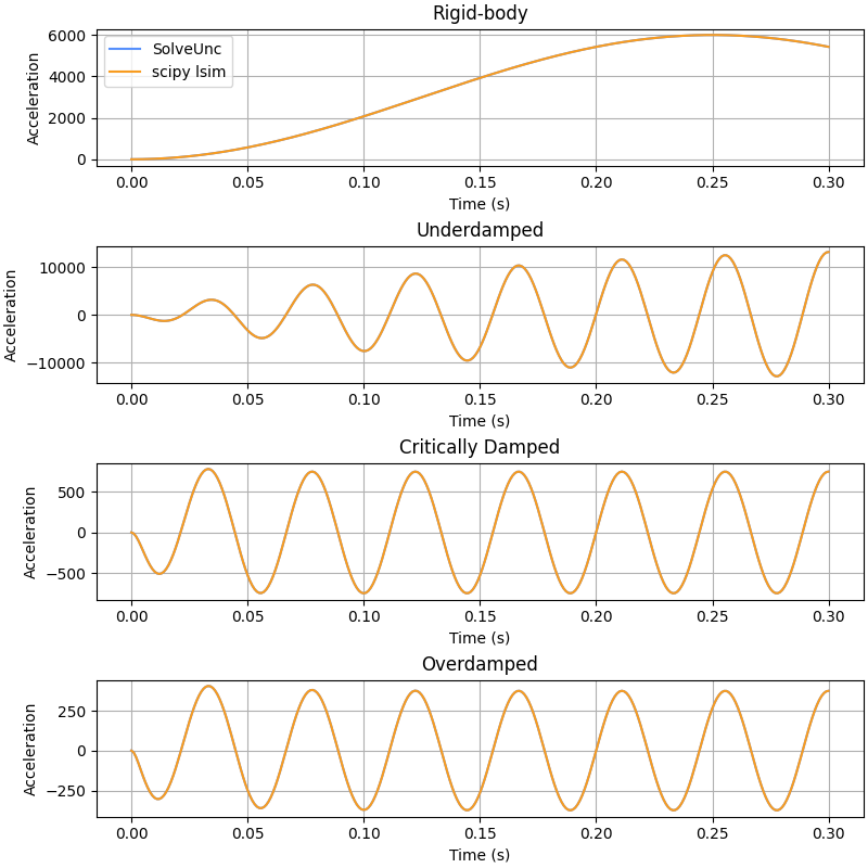
Plot the four accelerations:
>>> import matplotlib.pyplot as plt
>>> fig = plt.figure('Example', figsize=[8, 8], clear=True,
...                  layout='constrained')
>>> labels = ['Rigid-body', 'Underdamped',
...           'Critically Damped', 'Overdamped']
>>> for j, name in zip(range(4), labels):
...     _ = plt.subplot(4, 1, j+1)
...     _ = plt.plot(t, sol.a[j], label='SolveUnc')
...     _ = plt.plot(tl, yl[:, j], label='scipy lsim')
...     _ = plt.title(name)
...     _ = plt.ylabel('Acceleration')
...     _ = plt.xlabel('Time (s)')
...     if j == 0:
...         _ = plt.legend(loc='best')
- __init__(m, b, k, h=None, rb=None, rf=None, order=1, pre_eig=False, cd_as_force=False)[source]
Instantiates a
SolveUncsolver.- Parameters:
m (1d or 2d ndarray or None) – Mass; vector (of diagonal), or full; if None, mass is assumed identity
b (1d or 2d ndarray) – Damping; vector (of diagonal), or full
k (1d or 2d ndarray) – Stiffness; vector (of diagonal), or full
h (scalar or None; optional) – Time step; can be None if only want to solve a static problem or if only solving frequency domain problems
rb (1d array or None; optional) – Index or bool partition vector for rigid-body modes. Set to [] to specify no rigid-body modes. If None, the rigid-body modes will be automatically detected by this logic for uncoupled systems:
rb = np.nonzero(abs(k).max(0) < 0.005)[0]
And by this logic for coupled systems:
rb = ((abs(k).max(axis=0) < 0.005) &
      (abs(k).max(axis=1) < 0.005) &
      (abs(b).max(axis=0) < 0.005) &
      (abs(b).max(axis=1) < 0.005)).nonzero()[0]
Note
rb applies only to modal-space equations. Use pre-eig if necessary to convert to modal-space. This means that if rb is a partition vector, it specifies the rigid-body modes after the pre_eig operation. See also pre_eig.
rf (1d array or None; optional) – Index or bool partition vector for residual-flexibility modes; these will be solved statically. As for the rb option, the rf option only applies to modal space equations (possibly after the pre_eig operation).
order (integer; optional) – Specify which solver to use:
0 for the zero order hold (force stays constant across time step)
1 for the 1st order hold (force can vary linearly across time step)
pre_eig (bool; optional) – If True, an eigensolution will be computed with the mass and stiffness matrices to convert the system to modal space. This will allow the automatic detection of rigid-body modes which is necessary for the complex eigenvalue method to work properly on systems with rigid-body modes (unless those modes have damping). No modes are truncated. Only works if stiffness is symmetric/hermitian and mass is positive definite (see
scipy.linalg.eigh()). Just leave it as False if the equations are already in modal space.cd_as_force (bool; optional) – If damping is the only coupled matrix (after pre_eig if that is used), then setting this option to True means that:
The ODEs are solved with the diagonal terms only (this uses the standard pre-formulated integration coefficients from
get_su_coef()).The off-diagonal damping terms are treated as a force by moving them to the right-hand-side.
Note that the solution is not piece-wise linear exact in this case. The assumption is that the damping diagonal is dominant enough for the uncoupled solver coefficients to be good enough. A finer time-step may also be required. This option can be particularly advantageous when the generator (
SolveUnc.generator()) feature is used: in one test, using this option was approximately 70 times faster than the default (which uses the complex eigenvalue solution for coupled damping) and more than 200 times faster the theSolveExp2solver. In that test, the accuracy was acceptable with 25 points per cycle (ppc) at the highest frequency (ppc = 1 / (h * freq_high)). However, accuracy is problem dependent and needs to be verified before trusting the results.
Notes
The instance is populated with some or all of the following members. Note that in the table, non-rf/elastic means non-rf for uncoupled systems, elastic for coupled – the difference is whether or not the rigid-body modes are included in the final “k” matrix: they are for uncoupled but not for coupled.
Member
Description
m
mass for the non-rf/elastic modes
b
damping for the non-rf/elastic modes
k
stiffness for the non-rf/elastic modes
m_orig
original mass
b_orig
original damping
k_orig
original stiffness
h
time step
rb
index vector or slice for the rb modes
el
index vector or slice for the el modes
rf
index vector or slice for the rf modes
_rb
index vector or slice for the rb modes relative to the non-rf/elastic modes
_el
index vector or slice for the el modes relative to the non-rf/elastic modes
nonrf
index vector or slice for the non-rf modes
kdof
index vector or slice for the non-rf/elastic modes
n
number of total DOF
rbsize
number of rb modes
elsize
number of el modes
rfsize
number of rf modes
nonrfsz
number of non-rf modes
ksize
number of non-rf/elastic modes
invm
decomposition of m for the non-rf/elastic modes
imrb
decomposition of m for the rb modes
krf
stiffness for the rf modes
ikrf
inverse of stiffness for the rf modes
unc
True if there are no off-diagonal terms in any matrix; False otherwise
order
order of solver (0 or 1; see above)
pc
None or record (SimpleNamespace) of integration coefficients; if uncoupled, this is populated by
get_su_coef(); otherwise bySolveUnc.get_su_eig()pre_eig
True if the “pre” eigensolution was done; False otherwise
phi
the mode shape matrix from the “pre” eigensolution; only present if pre_eig is True
cdforces
True if cd_as_force option is being used (which means damping is coupled, but mass and stiffness are not)
bo
Off-diagonal damping terms (present when cdforces is True
systype
float or complex; determined by m b k
Unlike for
SolveExp2, order is not used until the solver is called. In other words, this routine prepares the integration coefficients for a first order hold no matter what the setting of order is, but the solver will adjust the use of the forces to account for the order setting.The mass, damping and stiffness may be real or complex since this solver is also used for frequency domain problems.
Methods
__init__(m, b, k[, h, rb, rf, order, ...])Instantiates a
SolveUncsolver.finalize([get_force])Finalize time-domain generator solution.
fsolve(force, freq[, incrb, rf_disp_only])Solve frequency-domain modal equations of motion using uncoupled equations.
generator(nt, F0[, d0, v0, static_ic])Python "generator" version of
SolveUnc.tsolve(); interactively solve (or re-solve) one step at a time.get_f2x(phi[, velo])Get force-to-displacement or force-to-velocity transform
get_su_eig(delcc)Does pre-calcs for the SolveUnc solver via the complex eigenvalue approach.
tsolve(force[, d0, v0, static_ic])Solve time-domain 2nd order ODE equations