pyyeti.srs.srs_frf

pyyeti.srs.srs_frf(frf, frf_frq, srs_frq, Q, *, getresp=False, return_srs_frq=None, scale_by_Q_only=False)

Compute SRS from frequency response functions.

Parameters:

• frf (2d array_like) – Columns of FRF data defining base motion in frequency domain: [FRF1, FRF2, … FRFn]. The FRFs can be complex; if so, this routine uses the absolute value of each column before interpolating to a frequency vector that includes system frequencies (note that using the absolute value gives equivalent results). Number of rows must equal len(frf_frq). If it is 1d, it is reshaped into a single column: [FRF1].

• frf_frq (1d array_like) – Frequency vector in Hz for the FRF data.

• srs_frq (1d array_like or None) – Frequency vector in Hz for the SRS. These are the SDOF frequencies for which to compute responses. If input as None, srs_frq depends on the scale_by_Q_only option:

  scale_by_Q_only	Description
  False (default)	srs_frq is computed from frf_frq such that the maximum theoretical response for the input at the FRF frequency is obtained. In this case, the computed SDOF frequency will be a little higher than the corresponding FRF frequency. How much higher depends on the damping: lower damping (higher Q) means the SDOF frequency will be closer to the FRF frequency. The equations are derived and discussed below.
  True	srs_frq is set equal to frf_frq

• Q (scalar) – Dynamic amplification factor \(Q = 1/(2\zeta)\) where \(\zeta\) is the critical damping ratio.

• getresp (bool; optional) – If True, return the complex response FRFs (see resp output below). Must be False if scale_by_Q_only is True.

• return_srs_frq (bool or None; optional) – Determines whether or not to return srs_frq:

  Setting	Description
  None	return_srs_frq will be internally reset to True if and only if the input srs_frq is None; otherwise, it is set to False
  True	Return srs_frq (default if srs_frq is None)
  False	Do not return srs_frq (default if srs_frq is not None)

• scale_by_Q_only (bool; optional) – Set to True to compute SRS as exactly Q * FRF instead of using the actual transfer function as shown below. This is discussed in some detail below in a “Note:” box in the Examples section. The parameter getresp must be False if scale_by_Q_only is True.

Returns:

• sh (2d ndarray) – The SRS results: [SRS1, SRS2, …. SRSn]; sh.shape = (len(srs_frq), n) where n is the number of FRFs.

• srs_frq (1d ndarray; optional) – The SRS frequency vector that goes with sh. See return_srs_frq description above.

• resp (dictionary; optional) – Only returned if getresp is True. Members:

  key	value
  ’freq’	frequency vector for responses; this is a superset of frf_frq and srs_frf with near-duplicates removed
  ’frfs’	3-D array; shape = (len(freq), n, len(srs_frq))
  ’srs_frq’	SRS frequency vector (here for convenience)

Notes

The shock response spectrum is the response of single DOF system(s) that are excited by an input base acceleration FRF:

  _____    ^
 |     |   |
 |  M  |  ---  SDOF response (x)
 |_____|
  /  |
K \ |_| C  ^
  /  |     |
[=======] ---  input base acceleration (frf)

The response of each system is computed independently by integration across the entire frequency range as specified in resp["freq"] above.

Derivation of the equation of motion follows. First, let:

\[\begin{split}\begin{aligned} \ddot{z} &= sig \\ M &= 1 \\ K &= \omega_n^2 \\ C &= 2\zeta\omega_n \\ \end{aligned}\end{split}\]

Note that \(\omega_n=2 \pi f_n\) where \(f_n\) is the natural frequency in Hz from the input srs_frq. The equation of motion is:

\[\begin{split}\begin{aligned} \ddot{x} &= \sum Forces\; on\; M \\ &= \omega_n^2(z-x)+2\zeta\omega_n(\dot{z}-\dot{x}) \end{aligned}\end{split}\]

Define a relative coordinate \(u = x - z\). Then:

\[\begin{split}\begin{aligned} \ddot{x}+2\zeta\omega_n\dot{u}+\omega_n^2 u &= 0 \\ \ddot{u}+2\zeta\omega_n\dot{u}+\omega_n^2 u &= -\ddot{z} \end{aligned}\end{split}\]

Using the Fourier transform \(\mathcal{F}[x(t)] = X(\Omega)\):

\[\begin{split}\begin{aligned} (-\Omega^2+2\zeta\omega_n\Omega j + \omega_n^2) U(\Omega) &= -Z_{acce}(\Omega) \\ U(\Omega) &= -Z_{acce}(\Omega) / (-\Omega^2+2\zeta\omega_n\Omega j + \omega_n^2) \\ U_{acce}(\Omega) &= \Omega^2 Z_{acce}(\Omega) / (-\Omega^2+2\zeta\omega_n\Omega j + \omega_n^2) \end{aligned}\end{split}\]

Then:

\[\begin{split}\begin{aligned} X_{acce}(\Omega) &= U_{acce}(\Omega) + Z_{acce}(\Omega) \\ &= \left ( \frac{\Omega^2} {\omega_n^2-\Omega^2+2\zeta\omega_n\Omega j} + 1 \right) Z_{acce}(\Omega) \end{aligned}\end{split}\]

The return value sh contains the peak of the absolute value of \(X_{acce}(\Omega)\) for all frequencies analyzed.

At what frequency is the amplitude of the transfer function maximized?

Letting \(p = \Omega / \omega_n\) and collecting terms, the transfer function is:

\[\begin{split}\begin{aligned} H(p) = \frac{X_{acce}(p)}{Z_{acce}(p)} &= \left ( \frac{p^2}{1-p^2+2\zeta p j} + 1 \right) \\ H(p) &= \left ( \frac{1 + 2\zeta p j}{1-p^2+2\zeta p j}\right) \end{aligned}\end{split}\]

If we just want the amplitude of the output over the input, multiply by the complex conjugate:

\[|H(p)|^2 = \left ( \frac{1 + (2\zeta p)^2}{(1-p^2)^2 +(2\zeta p)^2} \right)\]

For small damping values, the peak of \(|H(p)|\) occurs near \(p = 1\) (this is easy to see in the approximate expression below for the maximizing value of \(p\) (\(p_{peak}\))):

\[|H(p = 1)| = \sqrt{\frac{1}{(2\zeta)^2} + 1} = \sqrt{Q^2 + 1} \approx Q \text{ (for higher Q)}\]

To find precisely where \(|H(p)|^2\) is maximized, set the derivative with respect to \(p^2\) equal to zero and solve for \(p^2\) and then take the square root (sympy can be helpful here). The result is:

\[p_{peak} = \frac{\sqrt{ \sqrt{1 + 8 \zeta^2} - 1}}{2 \zeta} = Q \sqrt{ \sqrt{1 + 2 / Q^2} - 1}\]

A Taylor series expansion of \(p^2_{peak}\) was done to get the following very good approximate expression for \(p_{peak}\):

\[p_{peak} \approx \sqrt{1 - 2 \zeta^2} = \sqrt{1 - \frac{1}{2 Q^2}}\]

This routine uses the exact expression above for \(p_{peak}\) to add the maximizing analysis frequency for each SDOF:

\[\Omega_{peak} = p_{peak} \cdot \omega_n\]

It is important to note however that this will not necessarily maximize \(X_{acce}(\Omega)\) because that also depends on the input \(Z_{acce}(\Omega)\). If \(Z_{acce}(\Omega)\) is flat, then the above expression will maximize \(X_{acce}(\Omega)\). In the general case where \(Z_{acce}(\Omega)\) has a peak at a some frequency, to get the theoretical maximum SDOF response, the frequency of the SDOF (which is the srs_frq input to this routine) would need to be computed from:

\[\omega_n = \frac{\Omega}{p_{peak}}\]

Or, in terms of the input variable names:

\[srs{\_}frq = \frac{frf{\_}frq}{p_{peak}}\]

In this routine, to get the theoretical maximum SDOF response from a given \(Z_{acce}(\Omega)\), either compute srs_frq from the above equation before calling this routine or, alternatively, input srs_frq as None and let the routine internally perform that calculation.

Examples

Make up simple problem to demonstrate a couple of the equations derived above.

>>> import numpy as np
>>> from pyyeti import srs
>>> pk_input = 3.0
>>> pk_frq = 15.0
>>> frf = np.array([pk_input / 3, pk_input, pk_input / 3])
>>> frf_frq = np.array([pk_frq - 5, pk_frq, pk_frq + 5])
>>> srs_frq = np.array([pk_frq])
>>> Q = 20
>>> sh = srs.srs_frf(frf, frf_frq, srs_frq, Q)

Because the input has a peak at 15 hz and that is also the SDOF frequency, the peak response will occur at \(p = 1\) instead of \(p_{peak}\) as derived above. From the equations above, the absolute peak response should be: \(pk{\_}input \cdot \sqrt{Q^2 + 1}\):

>>> pk_should_be = pk_input * np.sqrt(Q ** 2 + 1)
>>> pk_should_be
60.074953183502359
>>> sh = srs.srs_frf(frf, frf_frq, srs_frq, Q)
>>> sh
array([[ 60.07495318]])
>>> abs(pk_should_be - sh[0, 0]) < 1e-10
True

If we let the routine compute the SDOF frequencies, we can get the theoretical maximum as derived above. Here, we’ll check both the peak response value and the frequency of the maximizing SDOF:

>>> p_peak = Q * np.sqrt((np.sqrt(1 + 2 / Q ** 2) - 1))
>>> frq_should_be = pk_frq / p_peak
>>> num = 1 + (p_peak / Q) ** 2
>>> den = (1 - p_peak ** 2) ** 2 + num - 1
>>> pk_should_be = pk_input * np.sqrt(num / den)
>>> sh, frq = srs.srs_frf(frf, frf_frq, None, Q)
>>> i = sh[:, 0].argmax()
>>> pk_should_be
60.093641865335883
>>> sh
array([[ 20.03121396],
       [ 60.09364187],
       [ 20.03121396]])
>>> abs(pk_should_be - sh[i, 0]) < 1e-10
True
>>> frq_should_be
15.009360389892359
>>> frq
array([ 10.00624026,  15.00936039,  20.01248052])
>>> abs(frq_should_be - frq[i]) < 1e-10
True

For the next example, the “equivalent sine” (SRS/Q) will be computed for a sawtooth input for several Q values.

Note

Since this is a pure sinusoidal analysis, one might think that the “equivalent sine” result should just be equal to the original input (and it will be, if scale_by_Q_only is True). However, because of excitation from nearby frequencies (as discussed in detail below), this will not be the case in general. Even so, depending on how the input was created, it may be valid to consider the input as the equivalent sine and set scale_by_Q_only to True. For example, if the input is an envelope over SDOF responses from time-domain signals, excitation from nearby frequencies may already be accounted for. Running this routine in that scenario with scale_by_Q_only set to False may just add unneeded conservatism.

Note

It is noted that with scale_by_Q_only set to False, dividing by \(\sqrt{Q^2 + 1}\) would make it more “equivalent” since that’s the gain of the transfer function at \(p = 1\) (see above). However, dividing by \(Q\) is common, and that’s what will be done for the example below.

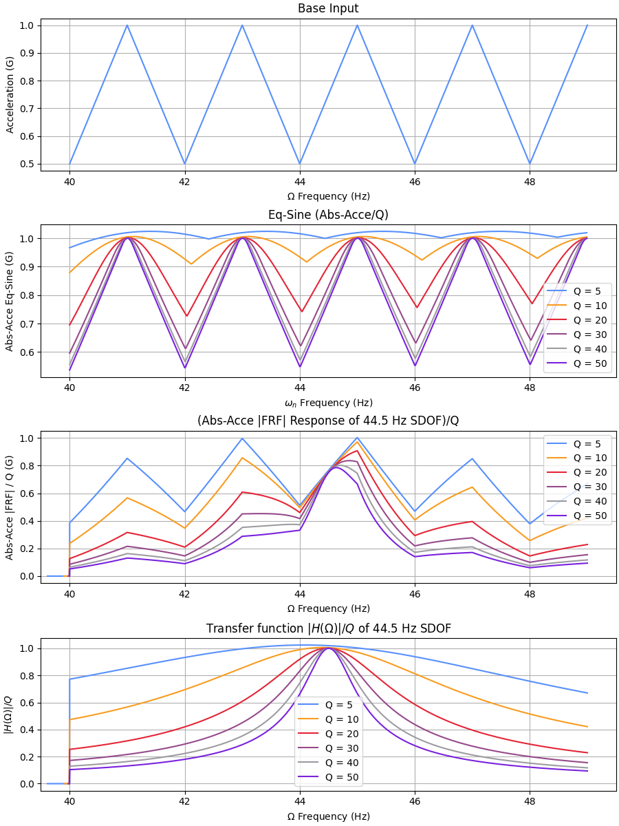
The top plot shows the input \(Z_{acce}(\Omega)\).

The second plot shows the equivalent sine curves for different damping values. Each curve has len(srs_frq) points on it, each point being the maximum value of \(|X_{acce}(\Omega)|/Q\) for the corresponding SDOF system.

The third plot shows the actual FRF response curves (divided by Q) for the 44.5 Hz SDOF system with the different damping values. The peak of each of these curves, at whatever frequency it occurs at, forms the corresponding value on the equivalent sine curve @ 44.5 Hz.

The fourth plot shows the transfer functions divided by Q for reference.

Observations (when scale_by_Q_only is False):

1. Equivalent sine curves with lower damping (higher Q), will tend to follow the input more closely. This is because the high gain of the transfer function near the SDOF natural frequency causes the response to hit its maximum peak near its natural frequency even if the peak of the input occurs at a different frequency. In that scenario, the division by Q (nearly) cancels out the gain of the transfer function, bringing the response back down to the input level. For example, for Q = 50, the FRF peak of the 44.5 Hz SDOF system occurs closest to the natural frequency even though the peak of the input does not occur there (the nearest input peak is at 45.0 Hz). So, the FRF peak is approximately Q * input.

2. Conversely, equivalent sine curves with higher damping (lower Q), will tend to smooth over the valleys of the input. For these higher damped SDOF systems, the lower gain of the transfer function becomes less important, and the peak response will occur closer to a peak of the input, even if that doesn’t match the natural frequency. For example, for Q = 5, the FRF peak of the 44.5 Hz SDOF system occurs at 45.0 Hz because that’s where the nearest peak of the input is. In that scenario, the division by Q will not bring the curve back down to the input level since the FRF peak is the product of off-peak transfer function (\(\neq Q\)) multiplied by a higher input at some other frequency. (Note: dividing by Q gets these curves closer to the input where the input has peaks, but still not as well as the lower damped equivalent sine curves … dividing by \(\sqrt{Q^2 + 1}\) would fix that.)

>>> import numpy as np
>>> import matplotlib.pyplot as plt
>>> from pyyeti import srs
>>>
>>> # saw tooth input:
>>> sdof = 44.5
>>> n = 10
>>> frf = np.ones(n)
>>> frf[::2] = 0.5
>>> frf_frq = np.arange(n) * 1.0 + 40.0
>>> srs_cutoff = frf_frq[-1]
>>> fstep = 0.01
>>>
>>> # add sdof frequency to frf_frq:
>>> new_frf_frq = np.sort(np.r_[frf_frq, sdof])
>>> new_frf = np.interp(new_frf_frq, frf_frq, frf)
>>> frf, frf_frq = new_frf, new_frf_frq
>>>
>>> srs_frq = np.arange(frf_frq[0], srs_cutoff, fstep)
>>>
>>> fig, ax = plt.subplots(
...     4,
...     1,
...     num="Example",
...     clear=True,
...     figsize=(9, 12),
...     layout='constrained',
... )
>>> _ = ax[0].plot(frf_frq, frf)
>>>
>>> for Q in (5, 10, 20, 30, 40, 50):
...     sh, resp = srs.srs_frf(
...         frf, frf_frq, srs_frq, Q, getresp=True
...     )
...     _ = ax[1].plot(srs_frq, sh / Q, label=f"Q = {Q}")
...     _ = ax[1].legend()
...
...     i = np.searchsorted(srs_frq, sdof)
...     _ = ax[2].plot(
...         resp["freq"],
...         abs(resp["frfs"][:, 0, i]) / Q,
...         label=f"Q = {Q}",
...     )
...     _ = ax[2].legend()
...
...     # plot the transfer function (by using unity input)
...     n = len(frf)
...     _, resp_unity = srs.srs_frf(
...         np.ones(n), frf_frq, srs_frq, Q, getresp=True
...     )
...     _ = ax[3].plot(
...         resp_unity["freq"],
...         abs(resp_unity["frfs"][:, 0, i]) / Q,
...         label=f"Q = {Q}",
...     )
...     _ = ax[3].legend()
>>>
>>> _ = ax[0].set_title("Base Input")
>>> _ = ax[0].set_ylabel("Acceleration (G)")
>>> _ = ax[0].set_xlabel(r"$\Omega$ Frequency (Hz)")
>>> _ = ax[1].set_title("Eq-Sine (Abs-Acce/Q)")
>>> _ = ax[1].set_ylabel("Abs-Acce Eq-Sine (G)")
>>> _ = ax[1].set_xlabel(r"$\omega_n$ Frequency (Hz)")
>>> _ = ax[2].set_title(
...         f"(Abs-Acce |FRF| Response of {sdof} Hz SDOF)/Q"
...     )
>>> _ = ax[2].set_ylabel("Abs-Acce |FRF| / Q (G)")
>>> _ = ax[2].set_xlabel(r"$\Omega$ Frequency (Hz)")
>>> _ = ax[3].set_title(
...         r"Transfer function $|H(\Omega)|/Q$ of "
...         f"{sdof} Hz SDOF"
...     )
>>> _ = ax[3].set_ylabel(r"$|H(\Omega)|/Q$")
>>> _ = ax[3].set_xlabel(r"$\Omega$ Frequency (Hz)")
>>> for axis in ax:
...    _ = axis.set_xlim(39.5, 49.5)

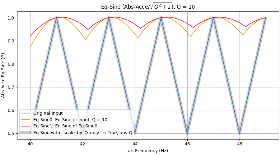
In the previous example, we saw that the equivalent sine of the input did not give us the original input back, but it was closer for lower damping. Fundamentally, the reason is because only the gain at \(p = 1\) is considered and, furthermore, the division by “Q” is an approximation of a more correct division by \(\sqrt{Q^2 + 1}\). An equivalent sine could get back to the original input if the original input was flat and the division was done using the theoretical maximum gain: \(|H(p=p_{peak})|\). (That assumes that the routine computing the SDOF responses catches the maximum gain frequency.)

So, how “equivalent” is the equivalent sine for the example shown above? In this final example, we’ll compute the equivalent sine of an equivalent sine for Q = 10. We’ll also improve the process a bit by dividing by \(\sqrt{Q^2 + 1}\) instead of Q. That will ensure that we get the values correct at the peak input frequencies. We’ll also include an equivalent sine curve created with the scale_by_Q_only option set to True; for this curve only, the division will be by Q.

>>> fig, ax = plt.subplots(
...     1,
...     1,
...     num="Example 2",
...     clear=True,
...     figsize=(9, 5),
...     layout='constrained',
... )
>>> _ = ax.plot(frf_frq, frf, label="Original Input")
>>>
>>> Q = 10
>>> factor = np.sqrt(Q ** 2 + 1)
>>>
>>> eqsine = srs.srs_frf(frf, frf_frq, srs_frq, Q) / factor
>>> lbl = f"Eq-Sine0; Eq-Sine of Input, Q = {Q}"
>>> _ = ax.plot(srs_frq, eqsine, label=lbl)
>>>
>>> for level in range(1):
...     eqsine = srs.srs_frf(
...         eqsine.ravel(), srs_frq, srs_frq, Q
...     ) / factor
...     lbl = f"Eq-Sine{level + 1}; Eq-Sine of Eq-Sine{level}"
...     _ = ax.plot(srs_frq, eqsine, label=lbl)
>>>
>>> eqsine = srs.srs_frf(
...     frf, frf_frq, srs_frq, Q, scale_by_Q_only=True
... ) / Q
>>> lbl = "Eq-Sine with `scale_by_Q_only` = True, any Q"
>>> _ = ax.plot(
...    srs_frq, eqsine, "k", linewidth=7, alpha=0.2, label=lbl
... )
>>>
>>> _ = ax.legend()
>>> _ = ax.set_title(
...    rf"Eq-Sine (Abs-Acce/$\sqrt{{Q^2+1}}$), Q = {Q}"
... )
>>> _ = ax.set_ylabel("Abs-Acce Eq-Sine (G)")
>>> _ = ax.set_xlabel(r"$\omega_n$ Frequency (Hz)")
>>> _ = ax.set_xlim(39.5, 49.5)