pyyeti.srs.srs

pyyeti.srs.srs(sig, sr, freq, Q, ic='zero', stype='absacce', peak='abs', ppc=12, rolloff='lanczos', eqsine=False, time='primary', getresp=False, parallel='auto', maxcpu=14)

Shock response spectrum - response of single DOF systems to base excitation(s).

Parameters:

• sig (1d or 2d array_like) – Base acceleration signal; vector or matrix where each column is a signal. If size is 1 x n (2d), that means there are n signals, each with length 1 (only initial conditions are calculated). For length 1 signal(s), you’ll probably want to set ic to ‘steady’.

• sr (scalar or None) – Sample rate. Can be None if signal(s) are length 1 and ic is not ‘zero’ (see note below).

• freq (1d array_like) – Frequency vector in Hz. This defines the single DOF systems to use.

• Q (scalar > 0.5) – Dynamic amplification factor \(Q = 1/(2\zeta)\) where \(\zeta\) is the fraction of critical damping. Q must be greater than 0.5 because this routine is for underdamped systems only.

• ic (string; optional) –

  Specifies how to handle the initial conditions:

  ic	Initial conditions
  ‘zero’	uses zero initial conditions
  ‘shift’	shifts each signal to start at zero so there are no step inputs and then uses zero initial conditions
  ‘mshift’	shifts each signal by its mean, then uses zero initial conditions
  ‘steady’	uses steady-state initial conditions

• stype (string; optional) –

  Specifies the type of response to recover:

  stype	Response that srs() calculates
  ‘absacce’	absolute acceleration
  ‘relacce’	relative acceleration
  ‘reldisp’	relative displacement
  ‘relvelo’	relative velocity
  ‘pvelo’	pseudo velocity (reldisp * omega)
  ‘pacce’	pseudo acceleration (reldisp * omega^2)

• peak (string or function; optional) –

  If a string, it must be one of these values:

  peak	Value the srs() returns
  ‘abs’	absolute maximum
  ‘pos’	maximum, absolute value
  ‘neg’	minimum, absolute value
  ‘poss’	maximum, keeping signs
  ‘negs’	minimum, keeping signs
  ‘rms’	root-sum-square

  If a function, it must accept the 2d response ndarray with shape = (len(time), nsignals) and return a 1d array of “peaks” with shape = (nsignals,). For example, the ‘abs’ function is:

  def _absmeth(resp):
      return abs(resp).max(axis=0)
  

• ppc (scalar; optional) – Specifies the minimum points per cycle for SRS calculations. See also rolloff.

  ppc	Maximum error at highest frequency
  3	81.61%
  4	48.23%
  5	31.58%
  10	8.14% (minimum recommended ppc)
  12	5.67%
  15	3.64%
  20	2.05%
  25	1.31%
  50	0.33%

• rolloff (string or function or None; optional) – Indicate which method to use to account for the SRS roll off when the minimum ppc value is not met. Either ‘fft’ or ‘lanczos’ seem the best. If a string, it must be one of these values:

  rolloff	Notes
  ‘fft’	Use FFT to upsample data as needed. See scipy.signal.resample().
  ‘lanczos’	Use Lanczos resampling to upsample as needed. See pyyeti.dsp.resample().
  ‘prefilter’	Apply a high freq. gain filter to account for the SRS roll-off. See preroll() for more information. This option ignores ppc [4].
  ‘linear’	Use linear interpolation to increase the points per cycle (this is not recommended; it’s only here as a test case).
  ‘none’	Don’t do anything to enforce the minimum ppc. Note error bounds listed above.
  None	Same as ‘none’.

  If a function, the call signature is: sig_new, sr_new = rollfunc(sig, sr, ppc, frq). sig is time x n. The last three inputs are scalars. For example, the ‘fft’ function is (trimmed of documentation):

  def fftroll(sig, sr, ppc, frq):
      N = sig.shape[0]
      if N > 1:
          curppc = sr/frq
          factor = int(np.ceil(ppc/curppc))
          sig = signal.resample(sig, factor*N, axis=0)
          sr *= factor
      return sig, sr
  

• eqsine (bool; optional) – If true, resulting history is divided by Q before the peak is extracted.

• time (string; optional) –

  Specifies the time-frame for SRS calculation:

  time	Time-frame for SRS calculation
  ‘primary’	During the signal(s) as input.
  ‘residual’	After the signal(s) (zeros are appended to allow one cycle of the lowest frequency).
  ‘total’	During and after the signal(s) (primary & residual).

• getresp (bool; optional) – If True, return the response time histories (see resp output below).

• parallel (string; optional) –

  Controls the parallelization of the SRS calculations:

  parallel	Notes
  ‘auto’	Routine determines whether or not to run parallel.
  ‘no’	Do not use parallel processing.
  ‘yes’	Use parallel processing. Beware, depending on the particular problem, using parallel processing can be slower than not using it (especially if getresp is True). On Windows, be sure the srs() call is contained within: if __name__ == "__main__":

• maxcpu (integer or None; optional) – Specifies maximum number of CPUs to use. If None, it is internally set to 4/5 of available CPUs (as determined from multiprocessing.cpu_count().

Returns:

• sh (1d or 2d ndarray) – The SRS results; sh.shape = (len(freq), nsignals). If sig is 1d, sh will also be 1d: sh.shape = (len(freq),).

• resp (dictionary; optional) – Only returned if getresp is True. Members:

  key	value
  ’t’	time vector for responses
  ’sr’	sample rate associated with ‘t’ (>= the input sr; depends on inputs sr, ppc, and rolloff)
  ’hist’	3-D array; shape = (len(t), nsignals, len(freq))

Notes

The shock response spectrum is the response of single DOF system(s) that are excited by an input base acceleration:

  _____    ^
 |     |   |
 |  M  |  ---  SDOF response (x)
 |_____|
  /  |
K \ |_| C  ^
  /  |     |
[=======] ---  input base acceleration (sig)

Derivation of the equation of motion follows. First, let:

\[\begin{split}\begin{aligned} \ddot{z} &= sig \\ M &= 1 \\ K &= \omega_n^2 \\ C &= 2\zeta\omega_n \\ \end{aligned}\end{split}\]

Note that \(\omega_n=2 \pi f_n\) where \(f_n\) is the natural frequency in Hz from the input freq. The equation of motion is:

\[\begin{split}\begin{aligned} \ddot{x} &= \sum Forces\; on\; M \\ &= \omega_n^2(z-x)+2\zeta\omega_n(\dot{z}-\dot{x}) \end{aligned}\end{split}\]

Define a relative coordinate \(u = x - z\). Then:

\[\begin{split}\begin{aligned} \ddot{x}+2\zeta\omega_n\dot{u}+\omega_n^2 u &= 0 \\ \ddot{u}+2\zeta\omega_n\dot{u}+\omega_n^2 u &= -\ddot{z} \end{aligned}\end{split}\]

In general, that equation is solved for each frequency for each signal, giving the relative displacement, velocity and acceleration. The absolute acceleration is then calculated from:

\[\ddot{x} = \ddot{u} + \ddot{z}\]

By assuming the input signal is linear between time points (ramp invariant), these equations can be solved in closed form. Reference [1] below has done this and conveniently put the solution in terms of linear digital filter coefficients. Furthermore, coefficients are provided to solve for whichever response is requested. More information on coefficient derivation can be found in references [2], and [3]. Reference [4] is a method for accounting for rolloff.

The maximum errors listed above are a summation of the bias error from the ramp invariant solver and the maximum error that can occur when selecting peaks (since peaks occur between solution points). The error equations are (noting that \(sr/f_n = ppc\)):

\[\begin{split}\begin{aligned} &\text{bias error} = 1 - \left[ \sin \left( \frac{\pi f_n}{sr} \right) / \frac{\pi f_n}{sr} \right]^2 \\ &\text{max peak error} = 1 - \cos \left( \frac{\pi f_n}{sr} \right) \end{aligned}\end{split}\]

Or:

\[\begin{split}\begin{aligned} &\text{bias error} = 1 - \left[ \sin \left( \frac{\pi}{ppc} \right) / \frac{\pi}{ppc} \right]^2 \\ &\text{max peak error} = 1 - \cos \left( \frac{\pi}{ppc} \right) \end{aligned}\end{split}\]

Note

The ‘zero’ and ‘mshift’ initial conditions may be handled in a slightly different manner than one might think: the zero initial displacement and velocity conditions occur one time step before sig begins (where sig is also assumed zero). This means one time step is analyzed even if the signal(s) are length 1; this is why sr cannot be None when ic = 'zero' (‘mshift’ is okay because it behaves like ‘shift’ when there is only one time step).

Note

In addition to the example shown below, this routine is demonstrated in the pyYeti Tutorials: SRS - the shock response spectrum. There is also a link to the source Jupyter notebook at the top of the tutorial.

References

[1]

“Mechanical vibration and shock – Signal processing – Part 4: Shock-response spectrum analysis”, ISO 18431-4.

[2]

Morin, A. and Labbé, P., “Derivation of Recursive Digital Filters by the Step-Invariant and the Ramp- Invariant Transformations”, DREV R-4325/84, May 1984, UNCLASSIFIED.

[3]

David Smallwood, “An Improved Recursive Formula for Calculating Shock Response Spectra”, 51st Shock and Vibration Bulletin (1980).

[4] (1,2)

Kjell Ahlin, “Shock Response Spectrum Calculation - An Improvement of the Smallwood Algorithm”, http://www.vibrationdata.com/tutorials/Ahlin_SRS.pdf

Raises:

• ValueError – When Q <= 0.5; routine is only for underdamped systems.

• ValueError – When sr is None but number of time steps is greater than 1 OR ic is set to ‘zero’.

Examples

>>> from pyyeti import srs
>>> import numpy as np
>>> sr = 1000.
>>> t = np.arange(0, 5, 1/sr)
>>> sig = np.sin(2*np.pi*15*t)
>>> Q = 20
>>> frq = [10, 15, 20]
>>> sh = srs.srs(sig, sr, frq, Q)
>>> print(f'{sh[1]:.1f}')
20.0

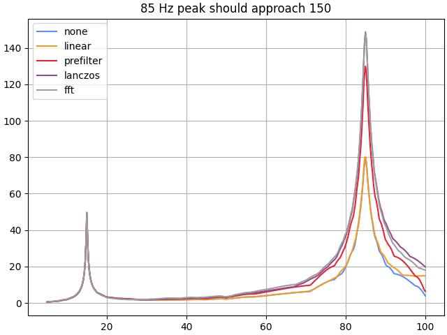
Compare the upsampling/rolloff methods:

>>> import matplotlib.pyplot as plt
>>> _ = plt.figure('Example', clear=True, layout='constrained')
>>> sr = 200
>>> t = np.arange(0, 5, 1/sr)
>>> sig = np.sin(2*np.pi*15*t) + 3*np.sin(2*np.pi*85*t)
>>> Q = 50
>>> frq = np.linspace(5, 100, 476)
>>> for meth in ['none', 'linear', 'prefilter',
...              'lanczos', 'fft']:
...    sh = srs.srs(sig, sr, frq, Q, rolloff=meth)
...    _ = plt.plot(frq, sh, label=meth)
>>> _ = plt.legend(loc='best')
>>> ttl = '85 Hz peak should approach 150'
>>> _ = plt.title(ttl)
>>> _ = plt.grid(True)