ode - time and frequency domain ODE solvers
This and other notebooks are available here: https://github.com/twmacro/pyyeti/tree/master/docs/tutorials.
Primarily, the pyyeti.ode module provides tools for solving 2nd order matrix equations of motion in both the time and frequency domains. This notebook demonstrates solving time-domain equations of motion.
Notes:
Some features depend on the equations being in modal space (particularly important where there are distinctions between the rigid-body modes and the elastic modes).
The time-domain solvers all depend on constant time step.
First, do some imports:
import numpy as np
import matplotlib.pyplot as plt
from pyyeti import ode
Some settings specifically for the jupyter notebook.
%matplotlib inline
plt.rcParams['figure.figsize'] = [6.4, 4.8]
plt.rcParams['figure.dpi'] = 150.
Setup a simple system
This system is not fixed to ground so it does have a rigid-body mode. This system is from the frclim.ntfl example.
        |--> x1       |--> x2        |--> x3        |--> x4
        |             |              |              |
     |----|    k1   |----|    k2   |----|    k3   |----|
 Fe  |    |--\/\/\--|    |--\/\/\--|    |--\/\/\--|    |
====>| 10 |         | 30 |         |  3 |         |  2 |
     |    |---| |---|    |---| |---|    |---| |---|    |
     |----|    c1   |----|    c2   |----|    c3   |----|
Define the mass, damping and stiffness matrices:
M1 = 10.
M2 = 30.
M3 = 3.
M4 = 2.
c1 = 15.
c2 = 15.
c3 = 15.
k1 = 45000.
k2 = 25000.
k3 = 10000.

MASS = np.array([[M1, 0, 0, 0],
                 [0, M2, 0, 0],
                 [0, 0, M3, 0],
                 [0, 0, 0, M4]])
DAMP = np.array([[c1, -c1, 0, 0],
                 [-c1, c1+c2, -c2, 0],
                 [0, -c2, c2+c3, -c3],
                 [0, 0, -c3, c3]])
STIF = np.array([[k1, -k1, 0, 0],
                 [-k1, k1+k2, -k2, 0],
                 [0, -k2, k2+k3, -k3],
                 [0, 0, -k3, k3]])
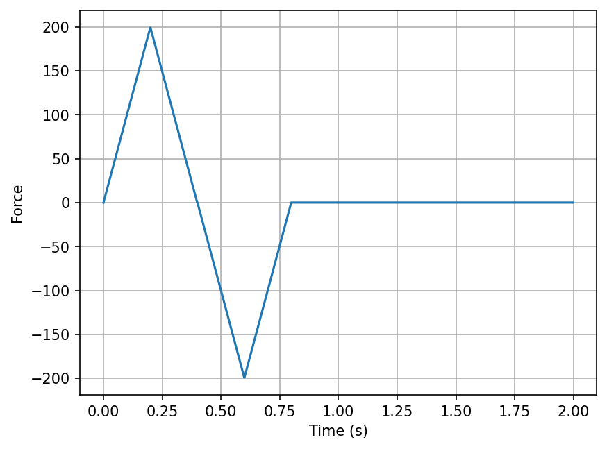
Define a time vector and a forcing function:
h = .001
t = np.arange(0, 2, h)
F = np.zeros((4, len(t)))
F[0, :200] = np.arange(200)
F[0, 200:400] = np.arange(200)[::-1]
F[0, 400:600] = np.arange(0, -200, -1)
F[0, 600:800] = np.arange(0, -200, -1)[::-1]
plt.plot(t, F[0])
plt.xlabel('Time (s)')
plt.ylabel('Force')
plt.grid(True)
The pyyeti.ode module was originally designed
only to solve systems that were in modal space via the
pyyeti.ode.SolveUnc
solver. Such equations are typically uncoupled, unless the damping is
coupled. This is an exact solver assuming piece-wise linear forces. For
the current problem, which is not in modal space, the solver now accepts
the pre_eig=True option which will internally transform the problem
to modal space.
You can also choose the
pyyeti.ode.SolveExp2
solver for the current problem. This solver is based on the matrix
exponential and is more general than
pyyeti.ode.SolveUnc.
For uncoupled equations however
pyyeti.ode.SolveUnc
is likely significantly faster. Note, even for the
pyyeti.ode.SolveExp2
solver, the equations will need to be put in modal space (via the
pre_eig=True) if you wish to use static initial conditions.
The pyyeti.ode.SolveUnc solver
Since this system is not in modal space, we’ll use the pre_eig=True.
ts = ode.SolveUnc(MASS, DAMP, STIF, h, pre_eig=True)
At this point, many pre-calculations are done and the ts object is
ready to be called (repeatedly if necessary) to solve the equations of
motion with arbitrary forces and initial conditions. The time domain
solver is called via the method
tsolve:
sol = ts.tsolve(F)
sol is a SimpleNamespace with the members:
.a - acceleration
.v - velocity
.d - displacement
.t - time vector
.h - time step
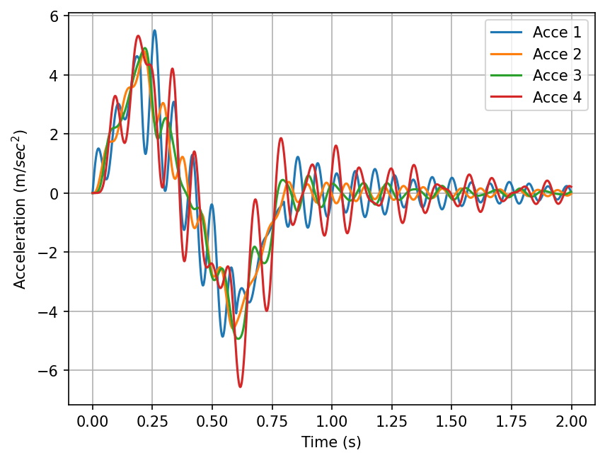
Plot the acceleration responses (assume metric units):
for j in range(sol.a.shape[0]):
    plt.plot(sol.t, sol.a[j], label='Acce {:d}'.format(j+1))
plt.legend(loc='best')
plt.xlabel('Time (s)')
plt.ylabel(r'Acceleration (m/$sec^2$)')
plt.grid(True)
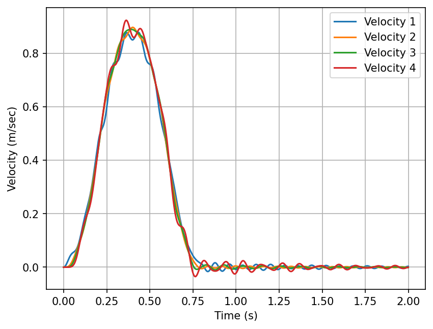
Plot the velocities:
for j in range(sol.v.shape[0]):
    plt.plot(sol.t, sol.v[j], label='Velocity {:d}'.format(j+1))
plt.legend(loc='best')
plt.xlabel('Time (s)')
plt.ylabel('Velocity (m/sec)')
plt.grid(True)
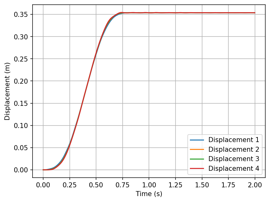
Plot the displacements:
for j in range(sol.d.shape[0]):
    plt.plot(sol.t, sol.d[j], label='Displacement {:d}'.format(j+1))
plt.legend(loc='best')
plt.xlabel('Time (s)')
plt.ylabel('Displacement (m)')
plt.grid(True)
The pyyeti.ode.SolveExp2 solver
For demonstration, we’ll solve the same system using the
pyyeti.ode.SolveExp2
solver. Since we’re not using static initial conditions, we don’t need
to use the pre_eig option. In this case, not using it would be more
efficient since it would do less work. For demonstration, we’ll use
both:
ts1 = ode.SolveExp2(MASS, DAMP, STIF, h)
ts2 = ode.SolveExp2(MASS, DAMP, STIF, h, pre_eig=True)
Solve with both solvers and demonstrate they give the same results:
sol1 = ts1.tsolve(F)
sol2 = ts2.tsolve(F)

assert np.allclose(sol1.a, sol2.a)
assert np.allclose(sol1.v, sol2.v)
assert np.allclose(sol1.d, sol2.d)
Show the results are also the same as the pyyeti.ode.SolveUnc solver:
assert np.allclose(sol1.a, sol.a)
assert np.allclose(sol1.v, sol.v)
assert np.allclose(sol1.d, sol.d)