pyyeti.cb.cbtf
- pyyeti.cb.cbtf(m, b, k, a, freq, bset, save=None)[source]
Compute frequency domain responses given i/f accel for a CB model.
- Parameters:
m (2d ndarray) – CB mass matrix. This routine does not assume the modal part is diagonal, but is assumed to be symmetric. Can be complex.
b (2d ndarray) – CB damping matrix. Modal part can be fully populated. Can be complex.
k (2d ndarray) – CB stiffness matrix. This routine does not assume the modal part is diagonal. Can be complex.
a (1d or 2d ndarray) – B-set acceleration to enforce; either bset x freq sized or a b-set length vector. If a b-set length vector, it is internally expanded and used for all frequencies. This is handy for constant (such as unity) base inputs.
freq (1d ndarray) – Frequency vector in Hz for solution.
bset (1d ndarray) – Index partition vector for the b-set; eg, np.arange(6)
save (None or dict; optional) – For efficiency. When using multiple a inputs, set save to an empty dict; this routine will put items in save to avoid unnecessary calculations.
- Returns:
A SimpleNamespace with the members
frc (complex 2d ndarray) – B-set force that was required to accelerate according to input a.
a (complex 2d ndarray) – B+Q-set accelerations (B-set part should match input a).
d (complex 2d ndarray) – B+Q-set displacements.
v (complex 2d ndarray) – B+Q-set velocities.
freq (1d ndarray) – The frequency vector (same as freq).
f (1d ndarray) – The frequency vector (same as freq … added for compatibility with the output of the ODE solvers in module
pyyeti.ode).
Notes
This routine is normally used to compute the transfer function by simply setting a equal to unity (or 1g) acceleration for the DOF of interest and zeros everywhere else.
This is analogous to doing a seismic mass baseshake, so the interface force F should have peaks at fixed-base Craig-Bampton frequencies. To exercise a free-free system, see
pyyeti.ode.SolveUncorpyyeti.ode.FreqDirect().The Craig-Bampton equations of motion in the frequency domain are:
\[\begin{split}\left[ \begin{array}{cc} M_{bb} & M_{bq} \\ M_{qb} & M_{qq} \end{array} \right] \left\{ \begin{array}{c} \ddot{X}_b(\Omega) \\ \ddot{X}_q(\Omega) \end{array} \right\} + \left[ \begin{array}{cc} B_{bb} & B_{bq} \\ B_{qb} & B_{qq} \end{array} \right] \left\{ \begin{array}{c} \dot{X}_b(\Omega) \\ \dot{X}_q(\Omega) \end{array} \right\} + \left[ \begin{array}{cc} K_{bb} & 0 \\ 0 & K_{qq} \end{array} \right] \left\{ \begin{array}{c} X_b(\Omega) \\ X_q(\Omega) \end{array} \right\} = \left\{ \begin{array}{c} F_b(\Omega) \\ 0 \end{array} \right\}\end{split}\]The input a is \(\ddot{X}_b(\Omega)\). Rearranging the bottom equation and using \(\dot{X}_b(\Omega)= -i\ddot{X}_b(\Omega)/\Omega\) gives:
\[\begin{split}\begin{aligned} M_{qq} \ddot{X}_q(\Omega) + B_{qq} \dot{X}_q(\Omega) + K_{qq} X_q(\Omega) &= -M_{qb} \ddot{X}_b(\Omega) - B_{qb} \dot{X}_b(\Omega) \\ &= \left(-M_{qb} + i B_{qb}/\Omega \right) \ddot{X}_b(\Omega) \end{aligned}\end{split}\]That equation is solved via
pyyeti.ode.SolveUnc.fsolve(). After solution, \(F_b(\Omega)\) is computed from the top equation above.Note
In addition to the example shown below, this routine is demonstrated in the pyYeti Tutorials: Checking data recovery matrices: modal DOF (cb.cbtf). There is also a link to the source Jupyter notebook at the top of the tutorial.
Examples
Use
cbtf()on a very simple 1-D spring mass CB component:[m1]--/\/\--[m2]--/\/\--[m3] <-- m1 is the bset DOF k1 k2 m1 = 4, k1 = 9000, m2 = 5, k2 = 3000, m3 = 7
>>> from pyyeti import cb
>>> import numpy as np
>>> import scipy.linalg as la
>>> import matplotlib.pyplot as plt
>>> np.set_printoptions(precision=4, suppress=True)
>>> m = np.array([[4, 0, 0], [0, 5, 0], [0, 0, 7]])
>>> k = np.array([[9000, -9000, 0], [-9000, 12000, -3000],
...              [0, -3000, 3000]])
Compute constraint modes and normal modes:
>>> psi = [1, 1, 1]
>>> w, phi = la.eigh(k[1:, 1:], m[1:, 1:])
Assemble CB transformation matrix, bset first:
>>> T = np.zeros((3, 3))
>>> T[:, 0] = psi
>>> T[1:, 1:] = phi
Compute CB mass and stiffness:
>>> mcb = T.T @ m @ T
>>> kcb = T.T @ k @ T
Make 3% modal damping matrix:
>>> zeta = .03
>>> bcb = np.diag(np.hstack((0, 2*zeta*np.sqrt(w))))
Set up frequency for solution and call
cbft():>>> outfreq = np.arange(.1, 10, .01) >>> tf = cb.cbtf(mcb, bcb, kcb, 1, outfreq, 0)
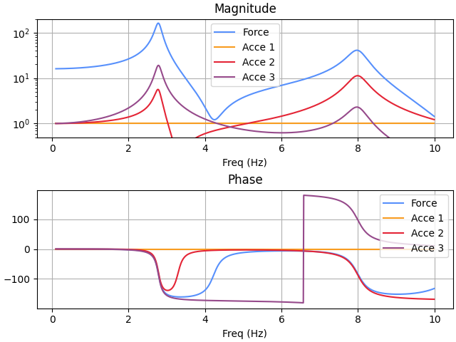
Recover physical accelerations and make some plots:
>>> a = T @ tf.a
>>> d = T @ tf.d
>>> fig = plt.figure('Example', clear=True,
...                  layout='constrained')
>>> ax = plt.subplot(211)
>>> lines = ax.plot(outfreq, np.abs(tf.frc).T, label='Force')
>>> lines += ax.plot(outfreq, np.abs(a).T)
>>> _ = ax.legend(lines,
...               ('Force', 'Acce 1', 'Acce 2', 'Acce 3'),
...               loc='best')
>>> _ = ax.set_title('Magnitude')
>>> _ = ax.set_xlabel('Freq (Hz)')
>>> ax.set_yscale('log')
>>> _ = ax.set_ylim([.5, 200])
>>> ax = plt.subplot(212)
>>> lines = ax.plot(outfreq, np.angle(tf.frc, deg=True).T)
>>> lines += ax.plot(outfreq, np.angle(a, deg=True).T)
>>> _ = ax.legend(lines,
...               ('Force', 'Acce 1', 'Acce 2', 'Acce 3'),
...               loc='best')
>>> _ = ax.set_title('Phase')
>>> _ = ax.set_xlabel('Freq (Hz)')