pyyeti.ode.SolveCDF

class pyyeti.ode.SolveCDF(m, b, k, h=None, rb=None, rf=None, order=1, pre_eig=False)

2nd order ODE time and frequency domain solvers for “uncoupled” equations of motion

This class is for solving:

\[M \ddot{q} + C \dot{q} + K q = P\]

This class inherits from SolveUnc and adds one additional time-domain solver for a special (but quite common) case: when damping is coupled but the mass and stiffness are diagonal. For all other cases, using SolveCDF is the same as using SolveUnc. In fact, all the coding for this solver is actually within the SolveUnc class. One can get to this solver by instantiating SolveUnc directly with the cd_as_force option set to True. So why does this class exist? For two reasons: one, to provide a consistent call signature with SolveUnc and SolveExp2, and two, as a convenient way to provide this documentation.

When the damping is coupled but the mass and stiffness are diagonal, this solver (SolveCDF) simply treats the off-diagonal damping terms as forces and uses the uncoupled equations (diagonal) solver of SolveUnc. “CDF” in the name stands for coupled damping forces. The procedure is outlined below.

Note that the solution is not piece-wise linear exact in this case. It is assumed that the off-diagonal damping terms for each ODE equation, in total, have a negligible effect on the derivative relationships for that equation and can be treated as applied forces. In practice, as long as the time-step is fine enough, this solver has been found to be fast and accurate.

SolveCDF can be particularly advantageous when the generator (SolveCDF.generator()) feature is used: in one test, using SolveCDF was approximately 70 times faster than using SolveUnc (which uses the complex eigensolution for coupled damping) and more than 200 times faster than the SolveExp2 solver. In that test, the accuracy was acceptable for SolveCDF with 25 points per cycle (ppc) at the highest frequency (ppc = 1 / (h * freq_high)). However, accuracy is problem-dependent and needs to be verified before the solution can be trusted.

Procedure

Consider the equations of motion with the off-diagonal damping terms moved to the right-hand-side to be treated as an applied force:

\[M \ddot{q} + C_d \dot{q} + K q = P - C_{od} \dot{q}\]

Since the ODE equations are uncoupled, the pre-formulated uncoupled integration coefficients are used (see get_su_coef()) as follows:

\[ \begin{align}\begin{aligned}\begin{array}{lr} \begin{aligned} q_{i+1} &= F q_i + G \dot{q}_i + A (P_i - C_{od} \dot{q}_i) + B (P_{i+1} - C_{od} \dot{q}_{i+1})\\ \dot{q}_{i+1} &= F_p q_i + G_p \dot{q}_i + A_p (P_i - C_{od} \dot{q}_i) + B_p (P_{i+1} - C_{od} \dot{q}_{i+1}) \end{aligned} \begin{aligned} \qquad \qquad (1&)\\ \qquad \qquad (2&) \end{aligned} \end{array}\end{aligned}\end{align} \]

Equation 2 can be solved for \(\dot{q}_{i+1}\):

\[ \begin{align}\begin{aligned}\begin{aligned} (I + B_p C_{od}) \dot{q}_{i+1} &= F_p q_i + G_p \dot{q}_i + A_p (P_i - C_{od} \dot{q}_i) + B_p P_{i+1}\\\dot{q}_{i+1} &= Z ( F_p q_i + G_p \dot{q}_i + A_p (P_i - C_{od} \dot{q}_i) + B_p P_{i+1})\\\dot{q}_{i+1} &= Z Vpart_i \end{aligned}\end{aligned}\end{align} \]

where \(Z = (I + B_p C_{od})^{-1}\) and \(Vpart_i = F_p q_i + G_p \dot{q}_i + A_p (P_i - C_{od} \dot{q}_i) + B_p P_{i+1}\).

With \(\dot{q}_{i+1}\), \(q_{i+1}\) can be computed from Equation 1 above. Using the equations as written, with \(Z\) precomputed, would require two matrix-vector multiplies per loop: \(Z Vpart_i\) and \(C_{od} \dot{q}_{i+1}\). We can get rid of one matrix-vector multiply per loop by precomputing the product of the two matrices outside the loop and reordering some calculations. First, precalculate \(\alpha\):

\[\alpha = C_{od} Z = C_{od} (I + B_p C_{od})^{-1}\]

Let the off-diagonal damping force be denoted by \(Q\) (\(Q_i \equiv C_{od} \dot{q}_i\)). Then, in the loop:

\[ \begin{align}\begin{aligned}\begin{aligned} Vpart_i &= F_p q_i + G_p \dot{q}_i + A_p (P_i - Q_i) + B_p P_{i+1}\\Q_{i+1} &= \alpha Vpart_i\\q_{i+1} &= F q_i + G \dot{q}_i + A (P_i - Q_i) + B (P_{i+1} - Q_{i+1})\\\dot{q}_{i+1} &= Vpart_i - B_p Q_{i+1} \end{aligned}\end{aligned}\end{align} \]

With that approach, there is only one matrix-vector multiply per loop: \(\alpha Vpart_i\).

Note

The above equations are for the non-residual-flexibility modes. The ‘rf’ modes are solved statically and any initial conditions are ignored for them.

For a static solution:

• rigid-body displacements = zeros

• elastic displacments = inv(k[elastic]) * P[elastic]

• velocity = zeros

• rigid-body accelerations = inv(m[rigid]) * P[rigid]

• elastic accelerations = zeros

See also

SolveUnc, SolveExp2

Examples

>>> from pyyeti import ode
>>> import numpy as np
>>> m = np.array([10., 30., 30., 30.])    # diag mass
>>> k = np.array([0., 6.e5, 6.e5, 6.e5])  # diag stiffness
>>> zeta = np.array([0., .05, 1., 2.])    # % damping
>>> b = np.diag(2.*zeta*np.sqrt(k/m)*m)   # diag of damping
>>> b_off = -np.diag(np.diag(b)[:-1], 1) / 100
>>> b += b_off + b_off.T                  # coupled damping
>>> h = 0.001                             # time step
>>> t = np.arange(0, .3001, h)            # time vector
>>> f = np.vstack((3*(1-np.cos(2*np.pi*2*t)),   # ffn
...                4.5*(np.cos(np.sqrt(k[1]/m[1])*t)),
...                4.5*(np.cos(np.sqrt(k[2]/m[2])*t)),
...                4.5*(np.cos(np.sqrt(k[3]/m[3])*t))))
>>> f *= 1.e4
>>> ts = ode.SolveCDF(m, b, k, h)
>>> sol = ts.tsolve(f, static_ic=1)

Solve with scipy.signal.lsim for comparison:

>>> A = ode.make_A(m, b, k)
>>> n = len(m)
>>> Z = np.zeros((n, n), float)
>>> B = np.vstack((np.eye(n), Z))
>>> C = np.vstack((A, np.hstack((Z, np.eye(n)))))
>>> D = np.vstack((B, Z))
>>> ic = np.hstack((sol.v[:, 0], sol.d[:, 0]))
>>> import scipy.signal
>>> f2 = (1./m).reshape(-1, 1) * f
>>> tl, yl, xl = scipy.signal.lsim((A, B, C, D), f2.T, t,
...                                X0=ic)
>>>
>>> print('acce cmp:',
...       np.allclose(yl[:, :n], sol.a.T,
...                   atol=1e-5*abs(sol.a).max()))
acce cmp: True
>>> print('velo cmp:',
...       np.allclose(yl[:, n:2*n], sol.v.T,
...                   atol=1e-5*abs(sol.v).max()))
velo cmp: True
>>> print('disp cmp:',
...       np.allclose(yl[:, 2*n:], sol.d.T,
...                   atol=1e-5*abs(sol.d).max()))
disp cmp: True

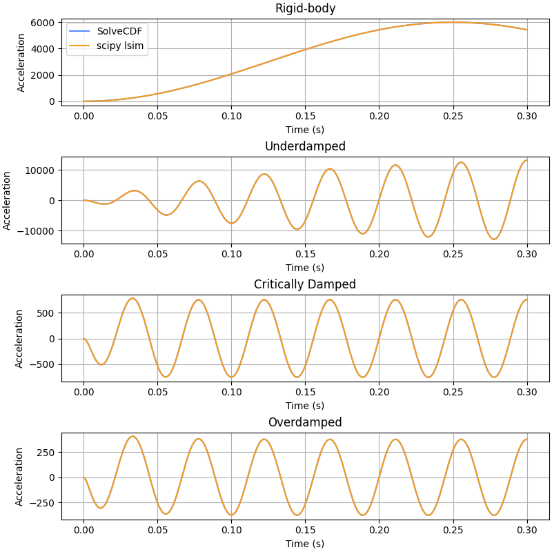
Plot the four accelerations:

>>> import matplotlib.pyplot as plt
>>> fig = plt.figure('Example', figsize=[8, 8], clear=True,
...                  layout='constrained')
>>> labels = ['Rigid-body', 'Underdamped',
...           'Critically Damped', 'Overdamped']
>>> for j, name in zip(range(4), labels):
...     _ = plt.subplot(4, 1, j+1)
...     _ = plt.plot(t, sol.a[j], label='SolveCDF')
...     _ = plt.plot(tl, yl[:, j], label='scipy lsim')
...     _ = plt.title(name)
...     _ = plt.ylabel('Acceleration')
...     _ = plt.xlabel('Time (s)')
...     if j == 0:
...         _ = plt.legend(loc='best')

__init__(m, b, k, h=None, rb=None, rf=None, order=1, pre_eig=False)

Instantiates a SolveCDF solver.

This simply calls SolveUnc.__init__() with the cd_as_force option set to True; see that function for more information.

Methods

__init__(m, b, k[, h, rb, rf, order, pre_eig])	Instantiates a SolveCDF solver.
finalize([get_force])	Finalize time-domain generator solution.
fsolve(force, freq[, incrb, rf_disp_only])	Solve frequency-domain modal equations of motion using uncoupled equations.
generator(nt, F0[, d0, v0, static_ic])	Python "generator" version of SolveCDF.tsolve(); interactively solve (or re-solve) one step at a time.
get_f2x(phi[, velo])	Get force-to-displacement or force-to-velocity transform
get_su_eig(delcc)	Does pre-calcs for the SolveUnc solver via the complex eigenvalue approach.
tsolve(force[, d0, v0, static_ic])	Solve time-domain 2nd order ODE equations