pyyeti.ode.SolveNewmark.def_nonlin

SolveNewmark.def_nonlin(dct)

Define nonlinear force terms

Parameters:

dct (dictionary) – Dictionary where each entry defines a nonlinear force term. You can define any number of terms. Each value is a sequence of 2 or 3 items: a function (or other callable), a 2d ndarray, and optionally a dictionary of arguments for the function. The dictionary keys are arbitrary but will be used as keys in the z return value in the output of tsolve(). The form of the dictionary is:

{
    key_0: (func_0, T_0 [, optargs_0]),
    key_1: (func_1, T_1 [, optargs_1]),
    ...
}

Item	Description
func_i	Each function must accept at least 3 arguments: the current solution displacement matrix (d), the current step index (j), and the time step (h). It can accept other arguments which are specified via optargs: def func_i(d, j, h [, ...]): The function must return a 1d ndarray. It will be multiplied by the corresponding transform T and added to the other force terms (this is the \(N_{n+1}\) term shown in SolveNewmark). See note below if velocity dependent terms are needed.
T_i	Each T_i matrix transforms the corresponding function output to a force. If your function outputs the final force already, just use identity for this transform. The reason this input is here, instead of relying on the user-supplied function func_i to apply the transform internally, is for efficiency: the relatively expensive operation of: \(A^{-1} T_i\) is precomputed outside the integration loop. The matrix \(A\) is defined in SolveNewmark.
optargs_i	If included, each optargs_i is a dictionary of arbitrary arguments for func_i.

Notes

The the j’th nonlinear force term is computed by:

N_j = (T_0 @ func_0(d, j, h, **optargs_0) +
       T_1 @ func_1(d, j, h, **optargs_1) +
       ...)

That term is used to compute the j+1’th displacement. That is appropriate because of the nature of the central finite difference formulae used in the Newmark-Beta formation. For reference, here is the equation (copied from SolveNewmark):

\[A u_{n+2} = \frac{1}{3} \left ( F_{n+2} + F_{n+1} + F_{n} \right ) + N_{n+1} + A_1 u_{n+1} + A_0 u_{n}\]

The solution namespace returned by tsolve() will contain the outputs of each user defined function in the dictionary z.

Note

Nastran estimates velocity by: \(v_j = (d_j - d_{j-1})/h\). In your function, you can use something like: vj = (d[:, j] - d[:, j-1])/h. That will work even for the first call, when j is 0, because “-1” displacements are stored in the last column of d for just this purpose.

Note

The nonlinear forces are computed in the integration loop for the non-residual flexibility equations only. Therefore, it is recommended to not use the rf option with nonlinear force terms.

Examples

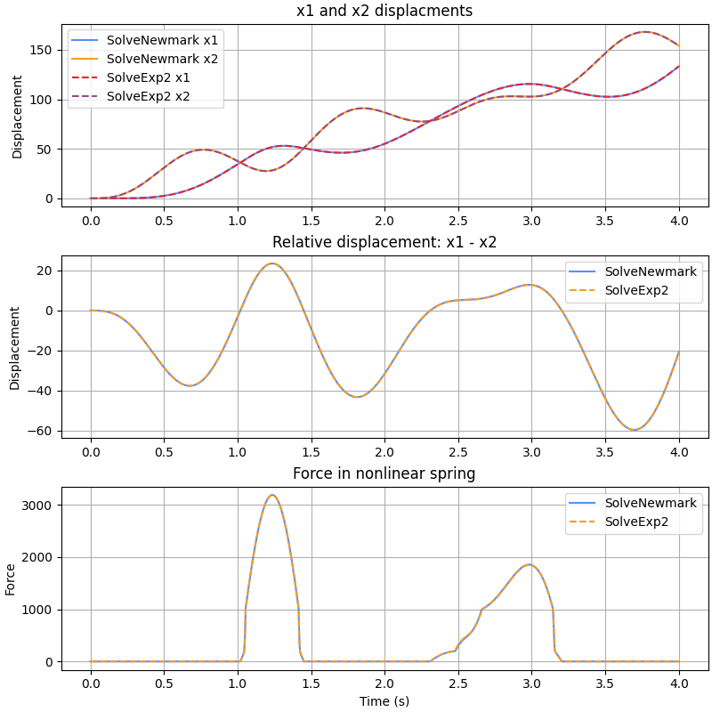
Model a two-mass system with one linear spring and one nonlinear spring. The nonlinear spring is only active when compressed. There is a gap of 0.01 units before the spring starts being compressed.

Model:

  |--> x1        |--> x2
|----|    50   |----|
| 10 |--\/\/\--| 12 |   F(t)
|    |         |    | =====>
|----| |-/\/-| |----|
     K_nonlinear

F(t) = 5000 * np.cos(2 * np.pi * t + 270 / 180 * np.pi)

The nonlinear spring force is linearly interpolated according to the “lookup” table below. Linear extrapolation is used for displacements out of range of the table.

>>> import numpy as np
>>> from scipy.interpolate import interp1d
>>> import matplotlib.pyplot as plt
>>> from pyyeti import ode
>>>
>>> # mass and stiffness:
>>> m = np.diag([10., 12.])
>>> k = np.array([[50., -50.],
...               [-50.,  50.]])
>>> c = 0. * k  # no damping
>>>
>>> # define time steps and force:
>>> h = 0.005
>>> t = np.arange(0, 4 + h / 2, h)
>>> f = np.zeros((2, t.size))
>>> f[1] = 5000 * np.cos(2 * np.pi * t + 3 / 2 * np.pi)
>>>
>>> # define interpolation table for force (the lookup
>>> # value is x1 - x2):
>>> lookup = np.array([[-10,     0.],
...                    [0.01,    0.],
...                    [5,     200.],
...                    [6,    1000.],
...                    [10,   1500.]])
>>>
>>> # for transforming lookup value to forces on the
>>> # masses:
>>> Tfrc = np.array([[-1.], [1.]])
>>>
>>> # turn interpolation table into a function for speed
>>> interp_func = interp1d(*lookup.T,
...                        fill_value='extrapolate')
>>>
>>> # function needed for ode.SolveNewmark.def_nonlin:
>>> def nonlin(d, j, h, interp_func):
...     return interp_func(d[[0], j] - d[[1], j])
>>>
>>> # Solve:
>>> ts = ode.SolveNewmark(m, c, k, h)
>>> ts.def_nonlin(
...     {'kcomp': (nonlin, Tfrc,
...               dict(interp_func=interp_func))})
>>> sol = ts.tsolve(f)
>>>
>>> # for comparison, run in SolveExp2 using the generator
>>> # feature:
>>> ts2 = ode.SolveExp2(m, c, k, h)
>>> gen, d, v = ts2.generator(len(t), f[:, 0])
>>>
>>> for i in range(1, len(t)):
...     if i == 1:
...         dx = d[0, i - 1] - d[1, i - 1]
...     else:
...         # for improved convergence, use linear
...         # interpolation to estimate displacements at
...         # current time:
...         dx = (2 * d[0, i - 1] - d[0, i - 2] +
...               d[1, i - 2] - 2 * d[1, i - 1])
...     f_nl = (Tfrc @ interp_func([dx]))
...     gen.send((i, f[:, i] + f_nl))
>>>
>>> sol2 = ts2.finalize()
>>>
>>> # plot results:
>>> _ = plt.figure('Example', figsize=(8, 8), clear=True,
...                layout='constrained')
>>>
>>> _ = plt.subplot(311)
>>> _ = plt.plot(t, sol.d.T)
>>> _ = plt.plot(t, d.T, '--')
>>> _ = plt.title('x1 and x2 displacments')
>>> _ = plt.ylabel('Displacement')
>>> _ = plt.legend(('SolveNewmark x1',
...                 'SolveNewmark x2',
...                 'SolveExp2 x1',
...                 'SolveExp2 x2'))
>>>
>>> _ = plt.subplot(312)
>>> _ = plt.plot(t, sol.d[0] - sol.d[1],
...              label='SolveNewmark')
>>> _ = plt.plot(t, d[0] - d[1], '--', label='SolveExp2')
>>> _ = plt.title('Relative displacement: x1 - x2')
>>> _ = plt.ylabel('Displacement')
>>> _ = plt.legend()
>>>
>>> _ = plt.subplot(313)
>>> _ = plt.plot(t, sol.z['kcomp'][0],
...              label='SolveNewmark')
>>> _ = plt.plot(t, interp_func(d[0, :] - d[1, :]), '--',
...              label='SolveExp2')
>>> _ = plt.title('Force in nonlinear spring')
>>> _ = plt.xlabel('Time (s)')
>>> _ = plt.ylabel('Force')
>>> _ = plt.legend()