pyyeti.ode.SolveNewmark
- class pyyeti.ode.SolveNewmark(m, b, k, h=None, rf=None)[source]
2nd order ODE time domain “Newmark-Beta” solver
This class is for solving:
\[M \ddot{u} + B \dot{u} + K u = F\]This routine uses a fixed time step Newmark-Beta method based on the Nastran Theoretical Manual, section 11.4 [1]. The algorithm is unconditionally stable but the size of the time step is still a concern for accurate results. According to Bathe [2], a time step that ensures accurate results for algorithms like this one is \(1/(80 f_{high})\), where \(f_{high}\) is the highest frequency (Hz) in your forcing functions.
In general, the mass, damping and stiffness can be fully populated (coupled).
Unlike
SolveUncandSolveExp2, this solver can handle a singular mass matrix. It can also handle non-linear force terms very well. For most (all?) other cases, the other two solvers are preferred since they are exact assuming piece-wise linear forces (if order is 1) or piece-wise constant forces (if order is 0).SolveUncis also very likely significantly faster for most problems.The equations for the non-residual equations are:
\[A u_{n+2} = \frac{1}{3} \left ( F_{n+2} + F_{n+1} + F_{n} \right ) + N_{n+1} + A_1 u_{n+1} + A_0 u_{n}\]where:
\[\begin{split}\begin{aligned} A &= \left [ \frac{M}{h^2} + \frac{B}{2 h} + \frac{K}{3} \right ] \\ A_1 &= \left [ \frac{2 M}{h^2} - \frac{K}{3} \right ] \\ A_0 &= \left [ \frac{-M}{h^2} + \frac{B}{2 h} - \frac{K}{3} \right ] \end{aligned}\end{split}\]\(N_{n+1}\) is a nonlinear force term which is optional; see
def_nonlin().To get the algorithm started, \(u_{-1}\) and \(F_{-1}\) are needed. They are computed from:
\[\begin{split}\begin{aligned} u_{-1} &= u_0 - \dot{u}_0 h \\ F_{-1} &= K u_{-1} + B \dot{u}_0 \end{aligned}\end{split}\]Also, \(F_0\) is replaced by:
\[F_{0} = K u_{0} + B \dot{u}_0\]According to [1], that is done to avoid ringing of massless degrees of freedom that are subjected to step loads. A side-effect of this is that \(\ddot{u}_0\) would be zero from the equation of motion. However, since the acceleration is computed from a central finite difference formula (see below), the resulting initial acceleration will not be zero in general. The acceleration values should be approximately correct by the third time step.
After the displacements have been calculated from the above equations, the velocities and accelerations are computed from:
\[\begin{split}\begin{aligned} \dot{u}_n &= \frac{1}{2 h} \left ( u_{n+1} - u_{n-1} \right ) \\ \ddot{u}_n &= \frac{1}{h^2} \left ( u_{n+1} - 2 u_n + u_{n-1} \right ) \end{aligned}\end{split}\]To compute the velocities and accelerations for the final time step, one extra integration step is performed by linearly extrapolating the force.
Note
The above equations are for the non-residual-flexibility modes. The ‘rf’ modes are solved statically and any initial conditions are ignored for them.
References
Examples
>>> from pyyeti import ode
>>> import numpy as np
>>> m = np.array([10., 30., 30., 30.])    # diag mass
>>> k = np.array([0., 6.e5, 6.e5, 6.e5])  # diag stiffness
>>> zeta = np.array([0., .05, 1., 2.])    # % damping
>>> b = 2.*zeta*np.sqrt(k/m)*m            # diag damping
>>> h = 0.0005                            # time step
>>> t = np.arange(0, 0.2, h)              # time vector
>>> c = 2*np.pi
>>> f = np.vstack((3*(1-np.cos(c*2*t)),   # ffn
...                4.5*(1 - np.cos(np.sqrt(k[1]/m[1])*t)),
...                4.5*(1 - np.cos(np.sqrt(k[2]/m[2])*t)),
...                4.5*(1 - np.cos(np.sqrt(k[3]/m[3])*t))))
>>> f *= 1.e4
>>> t2 = 2 / (np.sqrt(k[1] / m[1]) / 2 / np.pi)
>>> f[1:, t > t2] = 0.0
>>> nb = ode.SolveNewmark(m, b, k, h)
>>> sol = nb.tsolve(f)
Solve with
SolveUncfor comparison:>>> su = ode.SolveUnc(m, b, k, h) >>> solu = su.tsolve(f)
Check accuracy:
>>> for r in 'dva':
...     unc = getattr(sol, r)
...     new = getattr(solu, r)
...     atol = 0.01 * abs(unc).max()
...     print(r + ' comp:',
...           np.allclose(new, unc, atol=atol, rtol=0.001))
d comp: True
v comp: True
a comp: True
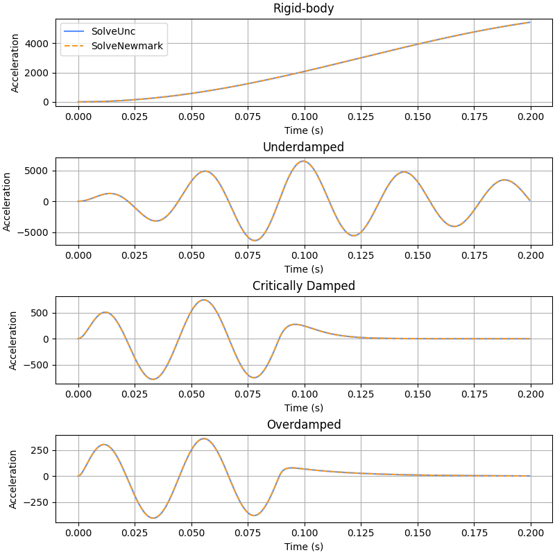
Plot the four accelerations:
>>> import matplotlib.pyplot as plt
>>> fig = plt.figure('Example', figsize=[8, 8], clear=True,
...                  layout='constrained')
>>> labels = ['Rigid-body', 'Underdamped',
...           'Critically Damped', 'Overdamped']
>>> for j, name in zip(range(4), labels):
...     _ = plt.subplot(4, 1, j+1)
...     _ = plt.plot(t, solu.a[j], label='SolveUnc')
...     _ = plt.plot(t, sol.a[j], '--', label='SolveNewmark')
...     _ = plt.title(name)
...     _ = plt.ylabel('Acceleration')
...     _ = plt.xlabel('Time (s)')
...     if j == 0:
...         _ = plt.legend(loc='best')
- __init__(m, b, k, h=None, rf=None)[source]
Instantiates a
SolveNewmarksolver.- Parameters:
m (1d or 2d ndarray or None) – Mass; vector (of diagonal), or full; if None, mass is assumed identity
b (1d or 2d ndarray) – Damping; vector (of diagonal), or full
k (1d or 2d ndarray) – Stiffness; vector (of diagonal), or full
h (scalar or None; optional) – Time step; can be None if only want to solve a static problem or if only solving frequency domain problems
rf (1d array or None; optional) – Index or bool partition vector for residual-flexibility modes; these will be solved statically. The rf option only applies to modal space equations.
Notes
The instance is populated with some or all of the following members.
Member
Description
m
mass for the non-rf DOF (or None for identity)
b
damping for the non-rf DOF
k
stiffness for the non-rf DOF
m_orig
original mass
b_orig
original damping
k_orig
original stiffness
h
time step
rb
np.array([])
el
index vector or slice for the non-rf DOF
rf
index vector or slice for the rf DOF
nonrf
index vector or slice for the non-rf DOF
kdof
index vector or slice for the non-rf DOF
n
number of total DOF
rbsize
0
elsize
number of non-rf DOF
rfsize
number of rf DOF
nonrfsz
number of non-rf DOF
ksize
number of non-rf DOF
krf
stiffness for the rf DOF
ikrf
inverse of stiffness for the rf DOF
unc
True if there are no off-diagonal terms in any matrix; False otherwise
systype
float or complex; determined by m b k
Ad
decomposed version of matrix \(A\) (see
SolveNewmark)A0
decomposed version of matrix \(A_0\)
A1
decomposed version of matrix \(A_1\)
nonlin_terms
number of nonlinear force terms defined by
def_nonlin()(initially set to 0)
Methods
__init__(m, b, k[, h, rf])Instantiates a
SolveNewmarksolver.def_nonlin(dct)Define nonlinear force terms
finalize([get_force])Finalize time-domain generator solution.
fsolve()'Abstract' method to solve frequency-domain equations
generator()'Abstract' method to get Python "generator" version of the ODE solver.
get_f2x()'Abstract' method to get the force to displacement transform used in Henkel-Mar simulations.
tsolve(force[, d0, v0])Solve time-domain 2nd order ODE equations