pyyeti.psd.psd2time
- pyyeti.psd.psd2time(spec, fstart, fstop, *, ppc=10, df=None, winends=None, gettime=False, expand_method='interp', rng=None)[source]
Generate a ‘random’ time domain signal given a PSD specification.
- Parameters:
spec (2d ndarray or 2-element tuple/list) – If ndarray, it has two columns:
[Freq, PSD]. Otherwise, it must be a 2-element tuple or list, eg:(Freq, PSD).fstart (scalar) – Starting frequency in Hz
fstop (scalar) – Stopping frequency in Hz
ppc (scalar; optional) – Points per cycle at highest (fstop) frequency; if < 2, it is internally reset to 2. With fstop, determines the sample rate:
sr = ppc * fstop.df (scalar or None; optional) – Serves two purposes: it is the frequency step between sinusoids included in the time signal, and it also determines the duration of the signal. If None, it is set to
fstart /
100
in order to have 100 cycles at the lowest frequency. If input as a scalar value, it is taken as a hint and will be internally adjusted lower as needed; see Notes section. If routine gives poor results, try refining df. If df is greater than fstart, it is reset internally to fstart (in that case though, you’ll only get 1 cycle at the lowest frequency). Total duration of the signal:T = 1 / df(see equations below for more details).Note
df can be used to indirectly specify the number of cycles desired at the lowest frequency (fstart). For example, if
fstart=5.0and you want to have 500 cycles of the 5.0 Hz content, then usedf=0.01:fstart / df == 500.winends (None or dictionary; optional) – If None,
pyyeti.dsp.windowends()is not called. Otherwise, winends must be a dictionary of arguments that will be passed topyyeti.dsp.windowends()(not including signal).gettime (bool; optional) – If True, a time vector is output.
expand_method (str; optional) – Either ‘interp’ or ‘rescale’, referring to which function in this module will be used to expand input spec to all needed frequencies. Use ‘interp’ if spec is a specification with constant dB/octave slopes. Use ‘rescale’ if spec provides the PSD levels on a center-band scale. See
interp()andrescale()for more information.rng (
numpy.random.Generatorobject or None; optional) – Random number generator. If None, a new generator is created vianumpy.random.default_rng(). Uniform deviates are generated viarng.random(). Supplying your own rng can be handy for parallel applications, for example, when you need repeatability. For illustration, the following creates a PCG-64 DXSM generator and initializes it with a seed of 1:from numpy.random import Generator, PCG64DXSM rng = Generator(PCG64DXSM(seed=1))
- Returns:
sig (1d ndarray) – The time domain signal with properties set to match input PSD spectrum. Duration of signal:
1 / df.sr (scalar) – The sample rate of the signal (
ppc * fstop)time (1d ndarray; optional) – Time vector for the signal starting at zero with step of
1.0 / sr:time = np.arange(len(sig)) / sr. Only returned if gettime is True.
Notes
The following outlines the equations used in this routine.
If \(df\) is None: \(df = fstart / 100\).
If \(df\) is greater than \(fstart\), it is reset to \(fstart\):
\[df = \min(df, fstart)\]The total time of the signal \(T\) is determined by the lowest frequency cycle (at frequency \(df\)):
\[T = 1 / df\]The number of points needed is determined by the number of cycles at the highest frequency multiplied by the points/cycle \(ppc\):
\[N = \lceil {fstop \cdot ppc \cdot T} \rceil\]The frequency step \(df\) is reset to match \(N\) (because of the possible round-up in the last equation):
\[df = fstop \cdot ppc / N\]The final downward adjustment to \(df\) is to make sure we hit the \(fstart\) frequency exactly:
\[df = fstart / \lfloor fstart / df \rfloor\]The frequency vector is defined by:
\[f = [fstart, fstart+df, ..., \lceil fstop / df \rceil \cdot df]\]A sinusoid is to be defined at each of those frequencies, so we need to compute an amplitude and phase for each.
The amplitude is determined by the magnitude of the PSD. Since a “power spectral density” is really mean-square spectral density, and since the mean-square value of a sinusoid is the amplitude squared over 2, the amplitude of each sinusoid is computed by:
\[amp(f) = \sqrt { 2 \cdot PSD(f) \cdot df }\]The phase is determined by using pseudo-random deviates from a uniform distribution:
\[phase(f) = U(0, 2\pi)\]The amplitude and phase are assembled together in a complex array so that an inverse-FFT will give a real time signal matching the desired mean-square profile defined by the input PSD.
- Raises:
ValueError – If more than one PSD specification is input.
ValueError – On invalid setting for expand_method.
See also
Examples
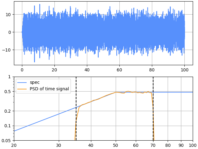
>>> import numpy as np
>>> from pyyeti import psd
>>> spec = np.array([[20,  .0768],
...                  [50,  .48],
...                  [100, .48]])
>>> we = dict(portion=0.01)
>>> seed = 1
>>> rng = np.random.default_rng(seed)
>>> sig, sr = psd.psd2time(
...     spec, 35, 70, ppc=10, df=.01, winends=we, rng=rng,
... )
>>> sr  # the sample rate should be 70*10 = 700
700.0
Compare the resulting psd to the spec from 37 to 68:
>>> import matplotlib.pyplot as plt
>>> import scipy.signal as signal
>>> f, p = signal.welch(sig, sr, nperseg=sr)
>>> pv = np.logical_and(f >= 37, f <= 68)
>>> fi = f[pv]
>>> psdi = p[pv]
>>> speci = psd.interp(spec, fi).ravel()
>>> abs(speci - psdi).max() < .05
True
>>> abs(np.trapezoid(psdi, fi) - np.trapezoid(speci, fi)) < .25
True
>>> fig = plt.figure('Example', clear=True,
...                  layout='constrained')
>>> a = plt.subplot(211)
>>> line = plt.plot(np.arange(len(sig))/sr, sig)
>>> plt.grid(True)
>>> a = plt.subplot(212)
>>> line = plt.loglog(spec[:, 0], spec[:, 1], label='spec')
>>> line = plt.loglog(f, p, label='PSD of time signal')
>>> leg = plt.legend(loc='best')
>>> x = plt.xlim(20, 100)
>>> y = plt.ylim(.05, 1)
>>> plt.grid(True)
>>> xticks = np.arange(20, 105, 10)
>>> x = plt.xticks(xticks, xticks)
>>> yticks = (.05, .1, .2, .5, 1)
>>> y = plt.yticks(yticks, yticks)
>>> v = plt.axvline(35, color='black', linestyle='--')
>>> v = plt.axvline(70, color='black', linestyle='--')