Using the pyYeti CLA tools
Introduction
Many thanks to Thomas Weber for his initial draft of this tutorial!
This and other jupyter notebooks are available here: https://github.com/twmacro/pyyeti/tree/master/docs/tutorials.
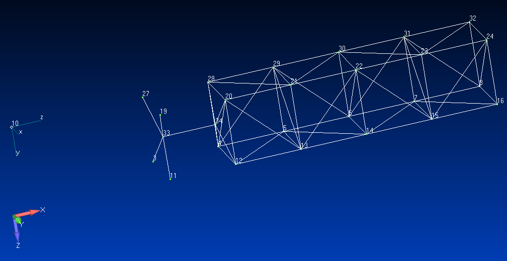
This tutorial will use a simple model to guide through the CLA process using the pyYeti tools. The model is a simple space station model contained in outboard.blk and inboard.blk. The outboard model will be used to create an external superelement, as if this model was delivered as a Craig-Bampton model by an independent group. The inboard model is the core of the residual structure. In the rocket launching business, the outboard model is analogous to a spacecraft model or an upstream component on the rocket, and the inboard model is analogous to the non-upstream part of the launch vehicle model.
Outboard:

outboard.png
Inboard:
inboard.png
Outline
The general outline for this tutorial is:
Outboard superelement creation
Prepare outboard model for CLA
Run modes on assembled model
Simulate loading events
Summarize results
Compare results
Special note about this tutorial
In order to speed up the automatic documentation creation step on “Read
the Docs”, a number of lines below are commented out. These all start
with # SPEED:. These lines all produce output that is not contained
within this notebook and would therefore only cost execution time while
creating the documentation. However, if you decide to run this tutorial
for yourself, it is recommended that these lines be uncommented so you
can take a look at all the output. Note that some screenshots of the
output is included below.
Nastran runs
The outboard model will be used to create an external superelement to
simulate a delivery from an independent team. The residual structure run
will bring in the outboard model as an external superelement as if we
did not have the bulk data. The inboard bulk data is included directly.
Both .dat files are shown below for convenience; they exist in the
srcdir directory that is shown below. These files were run in
Siemens Nastran version 2020.
import inspect
import os
from pathlib import Path
import pyyeti

srcdir = Path(inspect.getfile(pyyeti)).parent / "tests" / "cla_test_data_2020"
print(f"{srcdir = }")

wrkdir = Path.cwd()
print(f"{wrkdir = }")
srcdir = PosixPath('/home/docs/checkouts/readthedocs.org/user_builds/pyyeti/envs/stable/lib/python3.12/site-packages/pyyeti/tests/cla_test_data_2020')
wrkdir = PosixPath('/home/docs/checkouts/readthedocs.org/user_builds/pyyeti/checkouts/stable/docs/tutorials')
outboard.dat
The following Nastran input file creates the “outboard” external superelement (SE 101). This results in 3 files for use in the residual run: outboard.op4, outboard.asm, and outboard.pch.
In cases where a Craig-Bampton model is provided but the .op4, .asm, and .pch files are not provided, the routine pyyeti.nastran.bulk.wtextseout can be used to create these three files. This is typically done in the “prepare_4_cla.py” script shown below.
File “outboard.dat”:
INIT MASTER(S)  $ delete .MASTER and .DBALL files on exit
ASSIGN OUTPUT4='outboard.op4' UNIT=101,DELETE
SOL 103
CEND

TITLE = Outboard
ECHO = SORT
WEIGHTCHECK(SET=ALL) = YES
GROUNDCHECK(SET=ALL,DATAREC=YES) = YES
METHOD=1
SET 1 = 1 THRU 48
DISPLACEMENT(PLOT) = 1
FORCE(PLOT) = all
EXTSEOUT(ASMBULK,EXTBULK,EXTID=101,MATOP4=101)

BEGIN BULK
EIGRL          1            50.0
SPOINT   1995001    THRU 1995022
QSET1            1995001    THRU 1995022
BSET1,123456,3,11,19,27
include 'outboard.blk'
ENDDATA
residual.dat
Create the residual structure. This file uses inboard.blk and brings in SE 101 via the outboard.op4, outboard.asm and outboard.pch files. This run creates the nas2cam.op2 and nas2cam.op4 files that will be used for analysis in Python.
File “residual.dat”:
NASTRAN SYSTEM(402) = 0  $ AUTOMATICALLY DELETE DUPLICATE CARDS
NASTRAN NLINES = 10000
ASSIGN INPUTT4='outboard.op4',UNIT=101
INIT MASTER(S)  $ delete .MASTER and .DBALL files on exit
$ NAS2CAM op2/op4 files:
assign output2 = 'nas2cam.op2', status=new, unit=29,delete $
assign output4 = 'nas2cam.op4', status=new, unit=30,
     form=unformatted,delete $

DIAG    8,47
SOL 111
echooff
include '../nas2cam/nas2cam_111.v9'
include '../nas2cam/nas2cam_subdmap_2023.v9'

$ bug fix (?) alter for v2020:
COMPILE PHASE0
$ - delete line that prevents RVDOF from being used for resvecs
$ - must also include RESVEC(DYNRSP)=YES if need damping on these resvecs
ALTER 'IF ( NOT(RESVEC0) )'(2),'IF ( NOT(RESVEC0) )'(2) $ DELETE
$ Note: an alternative to RVDOF is to use the older PARAM,RESVEC,YES and
$ USET,U6 approach. That works without this little alter.
ENDALTER $

echoon
CEND

TITLE = System Modes
ECHO = Sort
METHOD = 1
FREQ = 1
DLOAD = 1
DISPLACEMENT(PLOT) = ALL
FORCE(PLOT) = ALL
WEIGHTCHECK(SET=ALL) = YES
GROUNDCHECK(SET=ALL,DATAREC=YES) = YES
RESVEC(NOAPPL,RVDOF,NORVEL,NOINRL,NODAMP,NODYNRSP)=YES

$-------------------------------------------------------------------
$ nas2cam params:
PARAM,PRFMODES,1
$
$ TO GENERATE GRAVITY FORCE, SET GRAVDIR EQUAL TO GRAVITY DIRECTION
$  AND SET THE GRAVITY FIELD:
$
PARAM,GRAVDIR,3
PARAM,GRAVFELD,9806.65  $ mm/sec**2
$-------------------------------------------------------------------

SUBCASE 1
    LABEL = Modes run with BHH matrix
    ANALYSIS = MODES

BEGIN BULK
$-------------------------------------------------------------------
$ NAS2CAM input:
PARAM,DBDICT,0
DTI,TMAA,1,101,0
DTI,TKAA,1,101,0
DTI,TGM,1,0
DTI,TPHG,1,0
DTI,TPHA,1,0
DTI,TBHH,1,0
$-------------------------------------------------------------------
PARAM,POST,-1
PARAM,SESDAMP,YES
EIGRL          1           150.0
$$$$$$$$$$$$$$$$$$$$$$$$$$$$$$$$$$$$$$$$$$$$$$$$
FREQ           1      2.
RLOAD2         1       1                       1
DAREA          1      11       1    1.0
TABLED1        1
            0.01     1.0   150.0    1.0     ENDT
$$$$$$$$$$$$$$$$$$$$$$$$$$$$$$$$$$$$$$$$$$$$$$$$
$ for residual flexibility vectors:
RVDOF1,123,8,22,24
INCLUDE 'outboard.asm'
include 'inboard.blk'
INCLUDE 'outboard.pch'
ENDDATA
Prepare Outboard for CLA
The prepare_4_cla.py file below prepares the outboard model for CLA. The primary goal is to setup data recovery.
This example also runs pyyeti.cb.cbcheck, though this could be done in a separate model checkout run. This is not discussed further here, but is the subject of a different tutorial: Using cb.cbcheck to check mass and stiffness.
A special data recovery category: “cglf”
The CG load factor category is special in that row 11 (at Python index 10) is a time-consistent RSS (root-sum-square) of rows 2 and 3. Rows 2 and 3 are the two 90 degrees apart shear-based lateral CG load factors in the SC coordinate system, so row 11 becomes the RSS shear-based lateral load factor. Similarly, row 12 is the RSS of 4 and 5, 13 is the RSS of 7 and 8, and 14 is the RSS of 9 and 10. Together, these rows cover both the shear-based and moment-based lateral CG load factors in the SC and LV coordinate systems. The corresponding RSS values for both coordinate systems should match each other. For PSD (power spectral density) analyses, an analogous RSS is handled with the help of pyyeti.cla.PSD_consistent_rss. The data recovery matrix for this category is created by pyyeti.cb.mk_net_drms and the last four rows (11-14) have only zeros.
To handle the RSS’ing during data recovery, the file “dr_file.py” is created for the “cglf” data recovery category with the routines “cglf” and “cglf_psd”. All the other data recovery categories are simple and handled directly in the “prepare_4_cla.py” file. See also pyyeti.cla.DR_Def.add for more details on creating data recovery categories.
For reference, the contents of “dr_file.py” are shown here:
import numpy as np
from pyyeti import cla


def get_xyr():
    # return the xr, yr, and rr indexes for the "cglf" data recovery
    xr = np.array([1, 3, 6, 8])  # 'x' row(s)
    yr = xr + 1  # 'y' row(s)
    rr = np.arange(4) + 10  # rss  rows
    return xr, yr, rr


def cglf(sol, nas, Vars, se):
    resp = Vars[se]["cglf"] @ sol.a
    xr, yr, rr = get_xyr()
    resp[rr] = np.sqrt(resp[xr] ** 2 + resp[yr] ** 2)
    return resp


def cglf_psd(sol, nas, Vars, se, freq, forcepsd, drmres, case, i):
    resp = Vars[se]["cglf"] @ sol.a
    cla.PSD_consistent_rss(resp, *get_xyr(), freq, forcepsd, drmres, case, i)
Miscellaneous notes regarding the “prepare_4_cla.py” file:
The dynamic uncertainty factor is set to 1.25
The SRS (shock response spectrum) is computed for some rows of some categories:
Q = 10 and 33
Frequency range from 0.1 to 50.0 Hz with step size 0.1 Hz
The SRS calculations are performed by pyyeti.srs.srs, pyyeti.srs.srs_frf, and pyyeti.srs.vrs for time-domain, frequency-domain, and PSD analyses, respectively.
All categories are added by using locally defined functions (all named “_”) and the pyyeti.cla.DR_Def.addcat decorator.
An elastic mode only “net_ifatm” category is added via pyyeti.cla.DR_Def.add_0rb. The name of the category will be “net_ifatm_0rb” (for zero rigid-body).
A summary of all categories is printed to an excel file “dr_summary.xlsx”. This is meant for visual checking and is shown below for reference.
Finally, the critical data is saved to “cla_params.pgz” via pyyeti.ytools.save. (Both pyyeti.ytools.save and pyyeti.ytools.load are imported into the “cla” module for convenience.)
# prepare_4_cla.py

from pathlib import Path
import numpy as np
import re
from pyyeti import cla, nastran, cb
from pyyeti.nastran import op4


def getlabels(lbl, id_dof):
    return ["{} {:4d}-{:1d}".format(lbl, g, i) for g, i in id_dof]


if __name__ == "__main__":
    se = 101
    uset, coords, bset = nastran.asm2uset(srcdir / "outboard.asm")
    bset = bset.nonzero()[0]
    dct = op4.read(srcdir / "outboard.op4")
    maa = dct["mxx"]
    kaa = dct["kxx"]
    atm = dct["mug1"]
    ltm = dct["mef1"]
    pch = srcdir / "outboard.pch"

    atm_labels = getlabels("Grid", nastran.rddtipch(pch, "tug1"))
    ltm_labels = getlabels("CBAR", nastran.rddtipch(pch, "tef1"))
    iflabels = getlabels("Grid", uset.index[bset])

    # setup CLA parameters:
    mission = "Micro Space Station"

    ref = [600.0, 150.0, 150.0]
    g = 9806.65
    net = cb.mk_net_drms(maa, kaa, bset, uset=uset, ref=ref, g=g)

    # run cbcheck:
    # SPEED: chk = cb.cbcheck(
    # SPEED:     "outboard_cbcheck.out", maa, kaa, bset, bref=np.arange(6), uset=uset, uref=ref
    # SPEED: )

    # define some defaults for data recovery:
    defaults = dict(
        se=se,
        uf_reds=(1, 1, 1.25, 1),
        srsfrq=np.arange(0.1, 50.1, 0.1),
        srsQs=(10, 33),
        drfile=srcdir / "dr_file.py"
    )

    drdefs = cla.DR_Def(defaults)

    @cla.DR_Def.addcat
    def _():
        name = "scatm"
        desc = "Outboard Internal Accelerations"
        units = "mm/sec^2, rad/sec^2"
        labels = atm_labels
        drms = {"atm": atm}
        drfunc = "Vars[se]['atm'] @ sol.a"
        # want translation histories and srs curves for nodes 35 & 36:
        prog = re.compile(" 3[56]-[123]")
        i = [i for i, s in enumerate(atm_labels) if prog.search(s)]
        histpv = np.zeros(len(labels), bool)
        histpv[i] = True
        srspv = histpv
        srsopts = dict(eqsine=1, ic="steady")
        drdefs.add(**locals())

    @cla.DR_Def.addcat
    def _():
        name = "scltm"
        desc = "Outboard Internal Loads"
        units = "mN, mN-mm"
        labels = ltm_labels
        drms = {"ltm": ltm}
        drfunc = "Vars[se]['ltm'] @ sol.d"
        drdefs.add(**locals())

    @cla.DR_Def.addcat
    def _():
        name = "ifatm"
        desc = "S/C Interface Accelerations"
        units = "mm/sec^2, rad/sec^2"
        labels = iflabels
        ifatm = np.eye(bset.shape[0], maa.shape[0])
        drms = {"ifatm": ifatm}
        drfunc = "Vars[se]['ifatm'] @ sol.a"
        srsopts = dict(eqsine=1, ic="steady")
        histpv = "all"
        drdefs.add(**locals())

    @cla.DR_Def.addcat
    def _():
        name = "ifltm"
        desc = "I/F Loads"
        units = "mN, mN-mm"
        labels = iflabels
        ifltma = maa[bset]
        ifltmd = kaa[bset][:, bset]
        drms = {"ifltma": ifltma, "ifltmd": ifltmd}
        drfunc = "Vars[se]['ifltma'] @ sol.a + Vars[se]['ifltmd'] @ sol.d"
        drdefs.add(**locals())

    @cla.DR_Def.addcat
    def _():
        name = "cglf"
        desc = "S/C CG Load Factors"
        units = "G"
        labels = net.cglf_labels
        drms = {"cglf": net.cglfa}
        histpv = slice(5)
        drdefs.add(**locals())

    @cla.DR_Def.addcat
    def _():
        name = "net_ifatm"
        desc = "NET S/C Interface Accelerations"
        units = "g, rad/sec^2"
        labels = net.ifatm_labels
        drms = {"net_ifatm": net.ifatm}
        drfunc = "Vars[se]['net_ifatm'] @ sol.a"
        srsopts = dict(eqsine=1, ic="steady")
        histpv = "all"
        drdefs.add(**locals())

    @cla.DR_Def.addcat
    def _():
        name = "net_ifltm"
        desc = "NET I/F Loads"
        units = "mN, mN-mm"
        labels = net.ifltm_labels
        drms = {"net_ifltm": net.ifltma}
        drfunc = "Vars[se]['net_ifltm'] @ sol.a"
        srsopts = dict(eqsine=0, ic="steady")
        histpv = "all"
        drdefs.add(**locals())

    # add a 0rb version of the NET ifatm:
    drdefs.add_0rb("net_ifatm")

    # make excel summary file for visual checking:
    # SPEED: drdefs.excel_summary("dr_summary.xlsx")

    # save data to gzipped pickle file:
    sc = dict(mission=mission, drdefs=drdefs)
    cla.save("cla_params.pgz", sc)

    print("Done!")
Done!
For reference, here is a screenshot of “dr_summary.xlsx”:

dr_summary.png
Run Events
There are 4 events run in this CLA: transfer orbit engine start (TOES), oil and water mixing experiment (OWLab), transfer orbit burn (TOBurn), and transfer orbit engine cutoff (TOECO). After these events are run, the results are summarized and compared.
First, for this tutorial, we’ll define a small convience function to ease running each event in it’s own subdirectory:
def set_event_dir(event):
    os.chdir(wrkdir)
    event_dir = Path(event)
    event_dir.mkdir(exist_ok=True)
    os.chdir(event_dir)
TOES
Outline of Transfer Orbit Engine Start run script:
Load data recovery data
Load Nastran data
Form ULVS for the outboard model (the SC)
ULVS is a row partition of the system modes to the superelement external DOF (typically the b-set and q-set DOF)
Prepare spacecraft data recovery matrices
Initialize results (ext, mnc, mxc for all drms)
Set rfmodes. This typically defines which modes are residual-flexibility modes, but really defines which modes are to be treated statically. See pyyeti.ode.SolveUnc for more information.
Setup modal mass, damping, and stiffness
Damping is diagonal, 2% modal damping
Load in forcing functions
Form force transform
Do ODE pre-calcs
Loop over all cases, solving the ODEs and performing data recovery
Compute the P99/90 statistical maximum and minimum values for each item
Save results and create tables and plots
Some screen shots of the tables and shown below for reference
set_event_dir("toes")
# Simulate event and recover responses
import numpy as np
from scipy.io import matlab
from pyyeti import stats, ode, cla
from pyyeti.nastran import n2p, op2


if __name__ == "__main__":
    # event name:
    event = "TOES"

    # load data recovery data:
    sc = cla.load(wrkdir / "cla_params.pgz")
    cla.PrintCLAInfo(sc["mission"], event)

    # load nastran data:
    nas = op2.rdnas2cam(srcdir / "nas2cam")

    # form ulvs for some SEs:
    SC = 101
    n2p.addulvs(nas, SC)

    # prepare spacecraft data recovery matrices
    DR = cla.DR_Event()
    DR.add(nas, sc["drdefs"])

    # initialize results (ext, mnc, mxc for all drms)
    results = DR.prepare_results(sc["mission"], event)

    # set rfmodes:
    rfmodes = nas["rfmodes"][0]

    # setup modal mass, damping and stiffness
    m = None  # None means identity
    k = nas["lambda"][0]
    assert nas["nrb"] == 6
    k[: nas["nrb"]] = 0.0
    b = 2 * 0.02 * np.sqrt(k)
    mbk = (m, b, k)

    # load in forcing functions:
    toes = matlab.loadmat(srcdir / "toes_ffns.mat", squeeze_me=True, struct_as_record=False)

    # form force transform:
    T = n2p.formdrm(nas, 0, [[8, 12], [24, 13]])[0].T

    # do pre-calcs and loop over all cases:
    ts = ode.SolveUnc(*mbk, 1 / toes["sr"], rf=rfmodes)
    LC = toes["ffns"].shape[0]
    t = toes["t"]
    for j, force in enumerate(toes["ffns"]):
        print("Running {} case {}".format(event, j + 1))
        genforce = T @ ([[1], [0.1], [1], [0.1]] * force[None, :])
        # solve equations of motion
        sol = ts.tsolve(genforce, static_ic=1)
        sol.t = t
        sol = DR.apply_uf(sol, *mbk, nas["nrb"], rfmodes)
        caseid = "{} {:2d}".format(event, j + 1)
        # perform data recovery:
        results.time_data_recovery(sol, nas["nrb"], caseid, DR, LC, j)

    # compute P99/90 statistical extreme values:
    results.calc_stat_ext(stats.ksingle(0.99, 0.90, LC))

    # save results:
    cla.save("results.pgz", results)

    # make some srs plots and tab files:
    # SPEED: results.rpttab()
    # SPEED: results.srs_plots()
    # SPEED: results.resp_plots()

    print("Done!")
Mission:  Micro Space Station
Event:    TOES
Running TOES case 1
Running TOES case 2
Running TOES case 3
Running TOES case 4
Running TOES case 5
Running TOES case 6
Running TOES case 7
Done!
For reference, here are some screenshots created by the above run:
The pyyeti.cla.DR_Results.rpttab routine writes tables of results. Here is a the “net_ifatm.tab” file (with some lines deleted for brevity). The extrema count table at the bottom shows that case 5 drove most of the “net_ifatm” extreme values.

toes_net_ifatm_tab.png
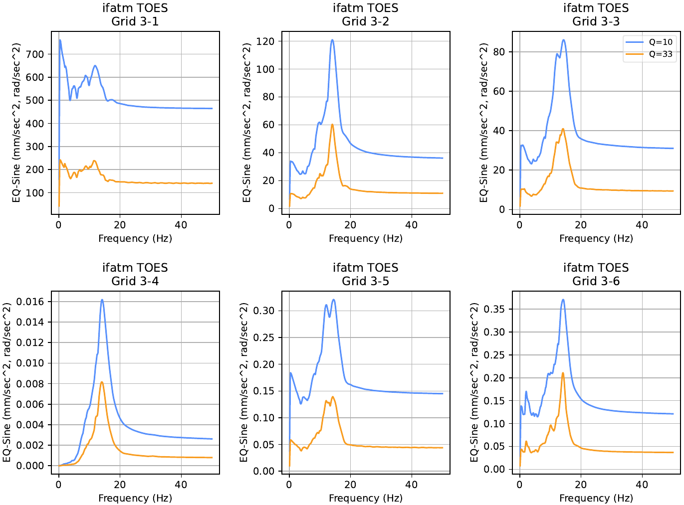
The pyyeti.cla.DR_Results.srs_plots routine plots all requested SRS curves to a file or files. Here is the first page of the “TOES_srs.pdf” file:
The pyyeti.cla.DR_Results.resp_plots routine plots all requested time-history curves to a file or files. Here is the first page of the “TOES_hist.pdf” file:
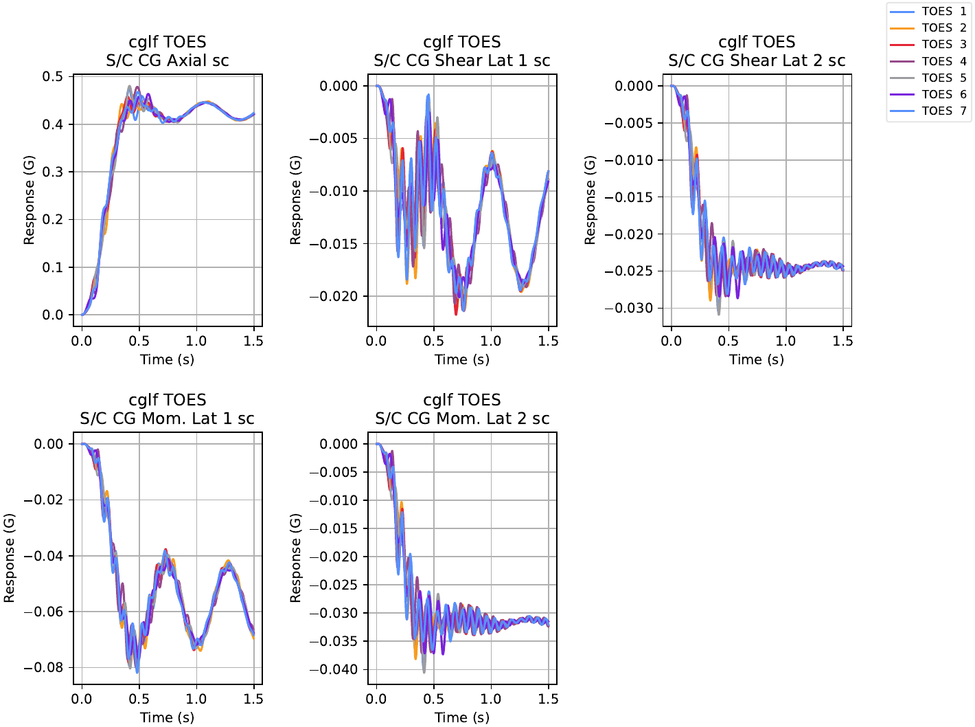
toes_hist_pg1.png
OWLab
Outline for oil and water mixing experiment:
Load data recovery data
Load Nastran data
Form ULVS for the outboard model (the SC)
Prepare spacecraft data recovery matrices
Initialize Results
Set rfmodes
Setup modal mass, damping, and stiffness
Damping is diagonal, 2% modal damping
Form force transform
Define the PSD forces
Calculate the PSD responses
Save results and make plots
Note:
We’ll see two warnings from this run, one about the frequency step being too large for accuracy, and another about a division by zero.
The first warning happens during the calculation of the SRS curves within the routine pyyeti.srs.vrs. For the integration frequency vector, this routine merges the frequencies from the forcing function, which range from 25 to 45 Hz by 0.5 Hz, with the frequencies at which to compute the SRS, which range from 0.1 to 50 Hz by 0.1 Hz. At the lowest frequencies then, the delta-frequency is 0.1 Hz which is larger than 0.1 / Q, so we get the warning. We could refine the SRS frequency vector in the prepare_4_cla step above to get rid of this warning. However, as noted in pyyeti.srs.vrs, the resulting SRS should be conservative and for this tutorial, this is acceptable. Additionally, in this case, we probably only care about the SRS in the 25 to 45 Hz range, which should be accurate.
The second warning happens during the calculation of the apparent frequency inside the pyyeti.cla.DR_Results.psd_data_recovery routine. The “scltm” has 4 zero rows and each of them will cause a divide-by-zero. For those rows, the “x” coordinate (which is normally the apparent frequency for PSDs) is set to NaN, which is perfectly fine.
set_event_dir("owlab")
# Simulate event and recover responses
import numpy as np
import scipy.interpolate as interp

from pyyeti import ode, cla
from pyyeti.nastran import n2p, op2


if __name__ == "__main__":
    # event name:
    event = "OWLab"

    # load data recovery data:
    sc = cla.load(wrkdir / "cla_params.pgz")
    cla.PrintCLAInfo(sc["mission"], event)

    # load nastran data:
    nas = op2.rdnas2cam(srcdir / "nas2cam")

    # form ulvs for some SEs:
    SC = 101
    n2p.addulvs(nas, SC)

    # prepare spacecraft data recovery matrices
    DR = cla.DR_Event()
    DR.add(nas, sc["drdefs"])

    # initialize results (ext, mnc, mxc for all drms)
    results = DR.prepare_results(sc["mission"], event)

    # set rfmodes:
    rfmodes = nas["rfmodes"][0]

    # setup modal mass, damping and stiffness
    m = None  # None means identity
    k = nas["lambda"][0]
    assert nas["nrb"] == 6
    k[: nas["nrb"]] = 0.0
    b = 2 * 0.02 * np.sqrt(k)
    mbk = (m, b, k)

    # form force transform:
    T = n2p.formdrm(nas, 0, [[22, 123]])[0].T

    # random part:
    freq = cla.freq3_augment(np.arange(25.0, 45.1, 0.5), nas["lambda"][0])
    rnd = [
        np.array(
            [
                # freq     x      y      z
                [1.0, 90.0, 110.0, 110.0],
                [30.0, 90.0, 110.0, 110.0],
                [31.0, 200.0, 400.0, 400.0],
                [40.0, 200.0, 400.0, 400.0],
                [41.0, 90.0, 110.0, 110.0],
                [50.0, 90.0, 110.0, 110.0],
            ]
        ),
        np.array(
            [
                # freq     x      y      z
                [1.0, 90.0, 110.0, 110.0],
                [20.0, 90.0, 110.0, 110.0],
                [21.0, 200.0, 400.0, 400.0],
                [30.0, 200.0, 400.0, 400.0],
                [31.0, 90.0, 110.0, 110.0],
                [50.0, 90.0, 110.0, 110.0],
            ]
        ),
    ]

    fs = ode.SolveUnc(*mbk, rf=rfmodes)
    for j, ff in enumerate(rnd):
        caseid = "{} {:2d}".format(event, j + 1)
        print("Running {} case {}".format(event, j + 1))
        F = interp.interp1d(ff[:, 0], ff[:, 1:].T, axis=1, fill_value=0.0)(freq)
        results.solvepsd(nas, caseid, DR, fs, F, T, freq)
        results.psd_data_recovery(caseid, DR, len(rnd), j)

    # save results:
    cla.save("results.pgz", results)

    # make some srs plots and tab files:
    # SPEED: results.rpttab()
    # SPEED: results.srs_plots(Q=10, direc="srs_cases", showall=True, plot="semilogy")
    # SPEED: results.resp_plots()

    print("Done!")
Mission:  Micro Space Station
Event:    OWLab
Running OWLab case 1
/home/docs/checkouts/readthedocs.org/user_builds/pyyeti/envs/stable/lib/python3.12/site-packages/pyyeti/srs.py:1353: RuntimeWarning: Integration frequency vector may produce inaccurate results; refine the step. See the documentation for more information.
  warn(
/home/docs/checkouts/readthedocs.org/user_builds/pyyeti/envs/stable/lib/python3.12/site-packages/pyyeti/cla/dr_results.py:1416: RuntimeWarning: invalid value encountered in divide
  pk_freq = vrms / rms
Running OWLab case 2
Done!
TOBURN
TOBurn is unique among the events analyzed in this tutorial because it uses a combination equation. There are two components: a “noise” component (solved in the PSD domain), and a steady-state thrust component (solved in the time-domain). The combination equation is simply the sum of these two components, noting that the noise component can be positive or negative.
Outline for Transfer Orbit Burn:
Define a function to combine the steady state burn with the noise of the burn
Load data recovery data
Load Nastran data
Form ULVS for the outboard model (the SC)
Prepare spacecraft data recover matrices
Initialize results
Set rfmodes
Setup modal mass, damping, and stiffness
Damping is diagonal, 2% modal damping
Form force transform
Calculate steady-state part
Calculate random part
Calculate combined results
Save results and Make plots
set_event_dir("toburn")
# Simulate event and recover responses
import numpy as np
import scipy.interpolate as interp
from pyyeti import ode, cla
from pyyeti.nastran import n2p, op2


def toburn_combine(event, results):
    """
    TOBurn combination equation

    Parameters
    ----------
    event: string
        Name to use for combined results; eg "TOBurn" (stored in, for
        example, ``results['combined']['SC_atm'].event``)
    results : instance of :class:`cla.DR_Results`
        Contains 'ss' and 'noise' instants of :class:`cla.DR_Results`.
        For example, if there is an "atm" category::

           results['ss']['atm']
           results['noise']['atm']

    Returns
    -------
    None

    Notes
    -----
    Adds the 'combined' instance of :class:`cla.DR_Results` to
    `results`.

    The combination equation is::

        mx = ss + noise
        mn = ss - noise
    """
    # use form_extreme to help form the combined results:
    results.form_extreme(ext_name=event)
    results["combined"] = results["extreme"]
    del results["extreme"]

    # now, just fix the "ext" members:
    for cat, sns in results["combined"].items():
        sns.domain = "combination"
        noise = results["noise"][cat]
        ss = results["ss"][cat]
        term = abs(noise.ext).max(axis=1)
        sns.ext[:, 0] = ss.ext[:, 0] + term
        sns.ext[:, 1] = ss.ext[:, 1] - term
        sns.exttime = None
        sns.maxcase = ["Combination"] * sns.ext.shape[0]
        sns.mincase = sns.maxcase
        # srs:
        if getattr(sns, "srs", None):
            _srs = sns.srs
            for Q in _srs.ext:
                _srs.ext[Q][:] = ss.srs.ext[Q] + noise.srs.ext[Q]


if __name__ == "__main__":
    # event name:
    event = "TOBurn"

    # load data recovery data:
    sc = cla.load(wrkdir / "cla_params.pgz")
    cla.PrintCLAInfo(sc["mission"], event)

    # load nastran data:
    nas = op2.rdnas2cam(srcdir / "nas2cam")

    # form ulvs for some SEs:
    SC = 101
    n2p.addulvs(nas, SC)

    # prepare spacecraft data recovery matrices
    DR = cla.DR_Event()
    DR.add(nas, sc["drdefs"])

    # initialize results (ext, mnc, mxc for all drms)
    results = cla.DR_Results()
    results["ss"] = DR.prepare_results(sc["mission"], event)
    results["noise"] = DR.prepare_results(sc["mission"], event)

    # set rfmodes:
    rfmodes = nas["rfmodes"][0]

    # setup modal mass, damping and stiffness
    m = None  # None means identity
    k = nas["lambda"][0]
    assert nas["nrb"] == 6
    k[: nas["nrb"]] = 0.0
    b = 2 * 0.02 * np.sqrt(k)
    mbk = (m, b, k)

    # form force transform:
    T = n2p.formdrm(nas, 0, [[8, 12], [24, 13]])[0].T

    # steady state part:
    case = "ss"
    ts = ode.SolveUnc(*mbk, rf=rfmodes)
    genforce = T @ [[7000.0], [0.0], [7000.0], [0.0]]
    sol = ts.tsolve(genforce, static_ic=1)
    sol = DR.apply_uf(sol, *mbk, nas["nrb"], rfmodes)
    results[case].time_data_recovery(sol, nas["nrb"], case, DR, 1, 0)

    # random part:
    case = "noise"
    freq = cla.freq3_augment(np.arange(5.0, 35.1, 0.5), nas["lambda"][0])
    F = interp.interp1d(
        [1.0, 50.0],
        [[300.0, 300.0], [30.0, 30.0], [350.0, 350.0], [35.0, 35.0]],
        axis=1,
        fill_value=0.0,
    )(freq)

    results[case].solvepsd(nas, case, DR, ts, F, T, freq)
    results[case].psd_data_recovery(case, DR, 1, 0)

    # combine results:
    toburn_combine(event, results)

    # save combined results:
    cla.save("results.pgz", results["combined"])

    # make some reports, plots:
    # SPEED: results["combined"].rpttab(excel=event.lower())
    # SPEED: results["combined"].srs_plots()

    # Plot SRS for Q=10 for ss, noise and combined:
    # SPEED: results["combined"].srs_plots(Q=10, direc="srs_cases", showboth=True)

    # Plot PSD response curves for the noise case
    # SPEED: results["noise"].resp_plots(plot="semilogy")

    print("Done!")
Mission:  Micro Space Station
Event:    TOBurn
/home/docs/checkouts/readthedocs.org/user_builds/pyyeti/envs/stable/lib/python3.12/site-packages/pyyeti/srs.py:1353: RuntimeWarning: Integration frequency vector may produce inaccurate results; refine the step. See the documentation for more information.
  warn(
/home/docs/checkouts/readthedocs.org/user_builds/pyyeti/envs/stable/lib/python3.12/site-packages/pyyeti/cla/dr_results.py:1416: RuntimeWarning: invalid value encountered in divide
  pk_freq = vrms / rms
Done!
For reference, here is the first page of the “TOBurn_psd.pdf” file (from pyyeti.cla.DR_Results.resp_plots):
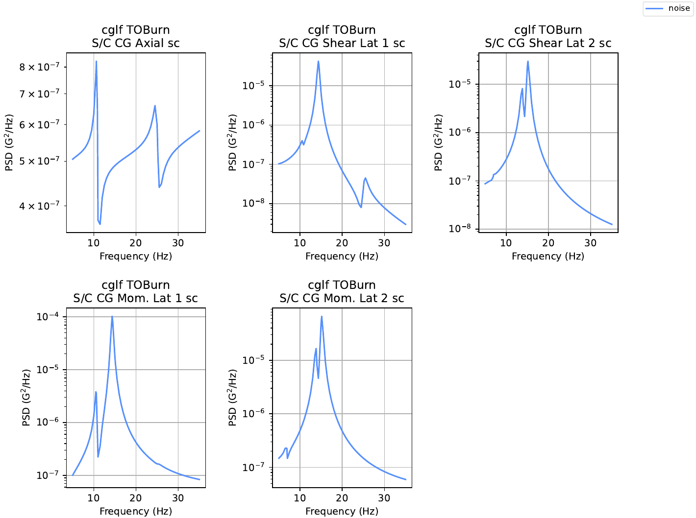
toburn_pg1.png
TOECO
Outline for Transfer Orbit Engine Cutoff:
Load data recovery data
Load nastran data
Form ULVS for the outboard model (the SC)
Prepare spacecraft data recovery matrices
Initialize results
Set rfmodes
Setup modal mass, damping, and stiffness
Damping is diagonal, 2% modal damping
Load in forcing functions
Form force transform
Do pre-calcs and loop over all cases
While looping, solve equations of motion
Save results and make plots
TOECO involves an acceleration recovery called “alphajoint”. The following file “alphajoint.py” facilitates setting up this category:
# alphajoint.py

import os
from pyyeti import cla
from pyyeti.nastran import n2p


def alphajoint(sol, nas, Vars, se):
    return Vars[se]["alphadrm"] @ sol.a


def get_drdefs(nas, sc):
    drdefs = cla.DR_Def(sc["drdefs"].defaults)

    @cla.DR_Def.addcat
    def _():
        se = 0
        name = "alphajoint"
        desc = "Alpha-Joint Acceleration"
        units = "mm/sec^2, rad/sec^2"
        labels = ["Alpha-Joint {:2s}".format(i) for i in "X,Y,Z,RX,RY,RZ".split(",")]
        drms = {"alphadrm": n2p.formdrm(nas, 0, 33)[0]}
        srsopts = dict(eqsine=1, ic="steady")
        histpv = 1  # second row
        srspv = [1]
        drfile = os.path.abspath(__file__)
        drdefs.add(**locals())

    return drdefs
set_event_dir("toeco")
# Simulate event and recover responses
import numpy as np
from scipy.io import matlab
from pyyeti import stats, ode, cla
from pyyeti.nastran import n2p, op2

import sys
sys.path.insert(0, os.path.abspath(srcdir))
import alphajoint


if __name__ == "__main__":
    # event name:
    event = "TOECO"

    # load data recovery data:
    sc = cla.load(wrkdir / "cla_params.pgz")
    cla.PrintCLAInfo(sc["mission"], event)

    # load nastran data:
    nas = op2.rdnas2cam(srcdir / "nas2cam")

    # form ulvs for some SEs:
    SC = 101
    n2p.addulvs(nas, SC)

    # prepare spacecraft and alphajoint data recovery matrices
    DR = cla.DR_Event()
    DR.add(nas, sc["drdefs"])
    DR.add(nas, alphajoint.get_drdefs(nas, sc))

    # initialize results (ext, mnc, mxc for all drms)
    results = DR.prepare_results(sc["mission"], event)

    # set rfmodes:
    rfmodes = nas["rfmodes"][0]

    # setup modal mass, damping and stiffness
    m = None  # None means identity
    k = nas["lambda"][0]
    assert nas["nrb"] == 6
    k[: nas["nrb"]] = 0.0
    b = 2 * 0.02 * np.sqrt(k)
    mbk = (m, b, k)

    # load in forcing functions:
    toeco = matlab.loadmat(srcdir / "toeco_ffns.mat", squeeze_me=True, struct_as_record=False)

    # form force transform:
    T = n2p.formdrm(nas, 0, [[8, 12], [24, 13]])[0].T

    # do pre-calcs and loop over all cases:
    ts = ode.SolveUnc(*mbk, 1 / toeco["sr"], rf=rfmodes)
    LC = toeco["ffns"].shape[0]
    t = toeco["t"]
    for j, force in enumerate(toeco["ffns"]):
        print("Running {} case {}".format(event, j + 1))
        genforce = T @ ([[1], [0.1], [1], [0.1]] * force[None, :])
        # solve equations of motion
        sol = ts.tsolve(genforce, static_ic=1)
        sol.t = t
        sol = DR.apply_uf(sol, *mbk, nas["nrb"], rfmodes)
        caseid = "{} {:2d}".format(event, j + 1)
        results.time_data_recovery(sol, nas["nrb"], caseid, DR, LC, j)

    # save results:
    cla.save("results.pgz", results)

    # make some srs plots and tab files:
    # SPEED: results.rpttab()
    # SPEED: results.srs_plots()
    # SPEED: results.resp_plots()

    print("Done!")
Mission:  Micro Space Station
Event:    TOECO
Running TOECO case 1
Running TOECO case 2
Running TOECO case 3
Done!
Take the data recovery information, spacecraft model, and forcing function to apply the event and save the results.
Summarize Results
os.chdir(wrkdir)
import numpy as np
from pyyeti import cla


if __name__ == "__main__":
    event = "Envelope"

    # load data in desired order:
    results = cla.DR_Results()
    results.merge(
        (
            cla.load(fn)
            for fn in [
                "toes/results.pgz",
                "owlab/results.pgz",
                "toburn/results.pgz",
                "toeco/results.pgz",
            ]
        ),
        {"OWLab": "O&W Lab"},
    )

    results.strip_hists()
    results.form_extreme(event, doappend=2)

    # save overall results:
    cla.save("summary_results.pgz", results)

    # write extrema reports:
    # SPEED: results['extreme'].rpttab()
    # SPEED: results['extreme'].rpttab(excel=event.lower())
    # SPEED: results['extreme'].srs_plots(Q=33, showall=True)

    print("Done!")
Done!
Here is the “net_ifatm.tab” file (with some lines deleted for brevity). The extrema count table at the bottom shows that TOBurn drove most of the “net_ifatm” extreme values.

ext_net_ifatm_tab.png
The pyyeti.cla.DR_Results.rpttab routine can also write the results tables to an excel file. In that case, extrema count pie charts are included. Here are the “scltm” pie charts:
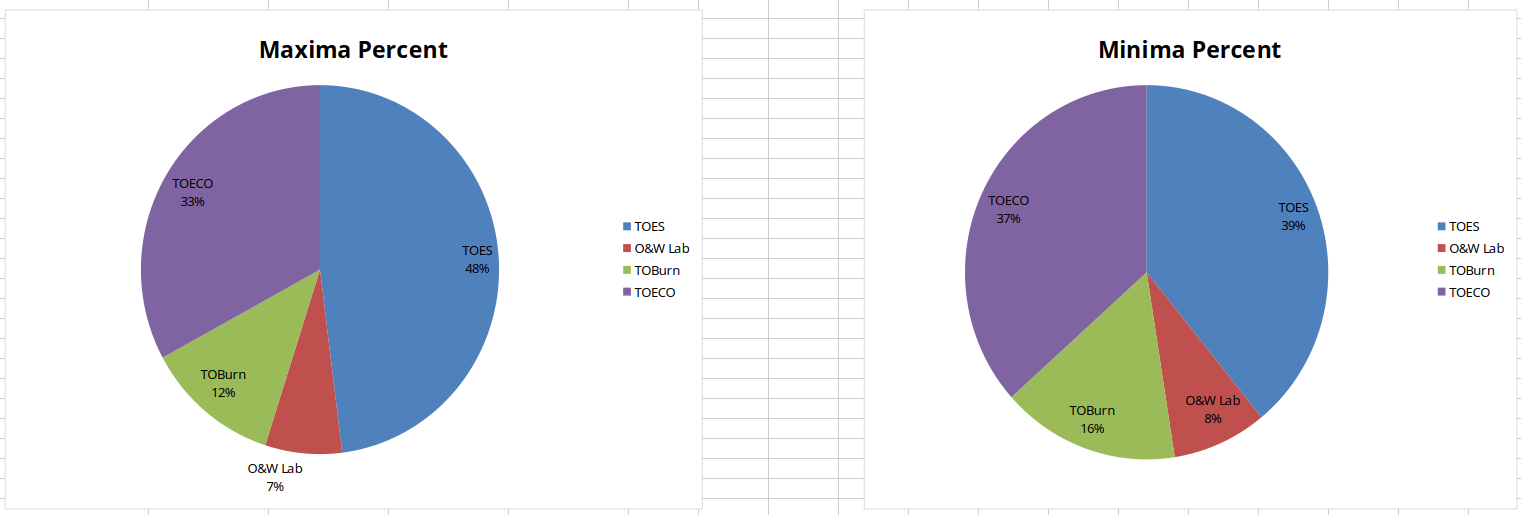
scltm_event_pie_chart.png
Grouping results:
The following is a brief demonstration of working with results contained in an pyyeti.cla.DR_Results instance.
This code groups the events into time domain events and frequency domain events, and plots some SRS’s for assessment:
# group results together to facilitate investigation:
Grouped_Results = cla.DR_Results()

# put these in the order you want:
groups = [
   ('Time Domain', ('TOES', 'TOECO')),
   ('Freq Domain', ('O&W Lab', 'TOBurn')),
]

for key, names in groups:
   Grouped_Results[key] = cla.DR_Results()
   for name in names:
       Grouped_Results[key][name] = results[name]

Grouped_Results.form_extreme()

# plot just time domain srs:
# SPEED: Grouped_Results['Time Domain']['extreme'].srs_plots(
# SPEED:    direc='timedomain_srs', Q=33, showall=True
# SPEED: )

# plot the srs of the two groups together:
# SPEED: Grouped_Results['extreme'].srs_plots(
# SPEED:    direc='grouped_srs', Q=33, showall=True
# SPEED: )

print("Done!")
Done!
Here is a page from the “grouped_srs/Envelope_srs.pdf” file:
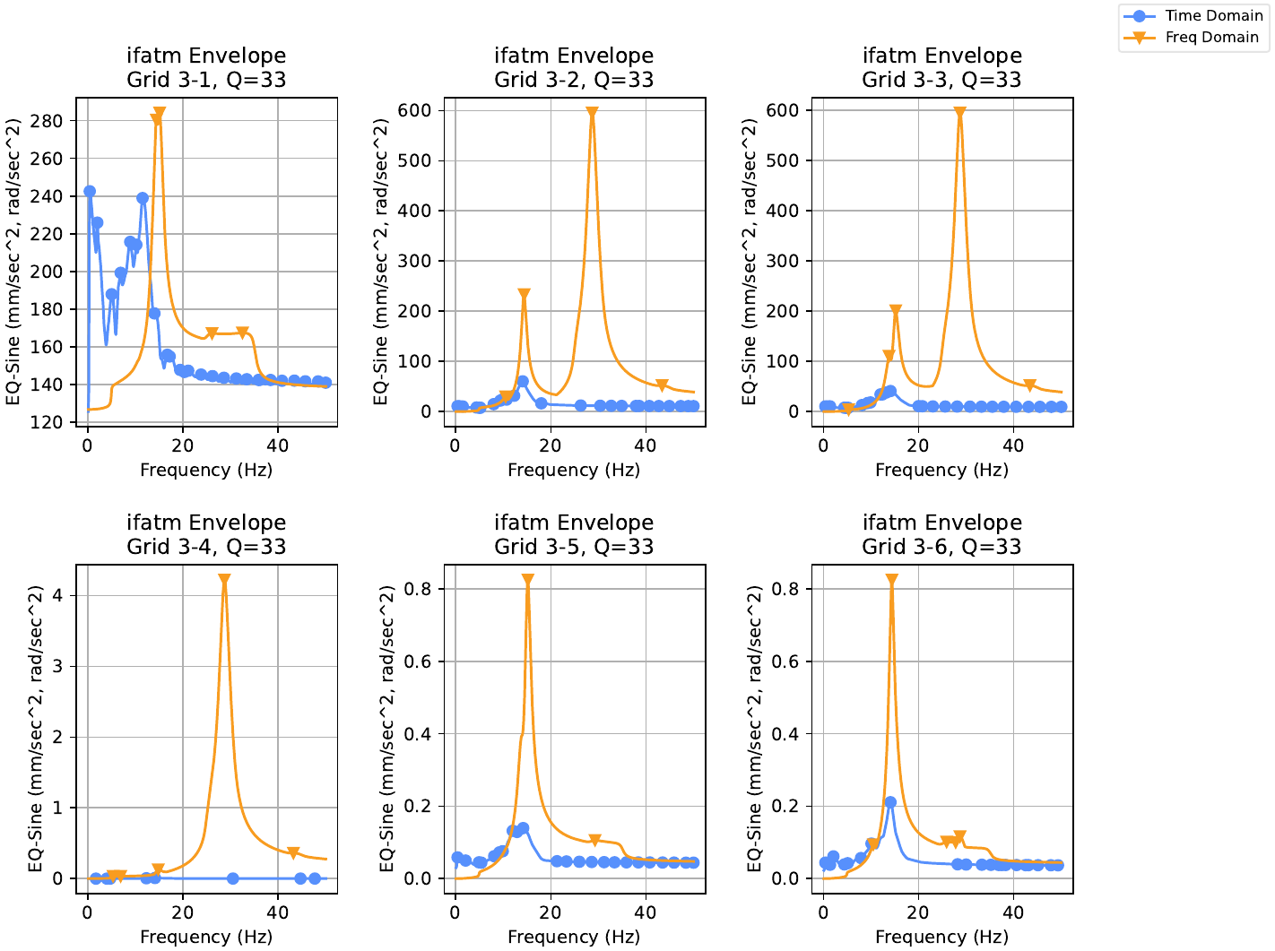
grouped_srs_ifatm_pg.png
Compare Results
Compare results generated here to those from the contractor:
import numpy as np
from pyyeti import cla
import pandas as pd


if __name__ == "__main__":
    results = cla.load("summary_results.pgz")
    lvc = pd.read_excel(srcdir / "contractor_results.xlsx", sheet_name=None, index_col=0)
    # SPEED: results['extreme'].rptpct(lvc, names=("Ours", "Theirs"), direc='compare')

    print("Done!")
Done!
For each category, pyyeti.cla.DR_Results.rptpct creates three files in the “compare” subdirectory: a .cmp file, a.cmp.histogram.png file, and a *.cmp.magpct.png file. Examples from the “net_ifatm” category follow.
Here is a the top of the “net_ifatm.cmp” file. The table at the top has the detailed comparison of maximums, minimums, and absolute-maximums. There are accompanying comparison histogram counts with statistics for each of these at the bottom (here, for brevity, only the maximums histogram data is shown). All “net_ifatm” maximums are within 3%, and 75% of maximums are within 1%.

cmp_net_ifatm_tab.png
Here is the “net_ifatm.cmp.histogram.png” file which shows the histogram data in a bar plot format. Bars within 5% are shown in blue, bars from 5 to 10% are purple, and bars above 10% are red.
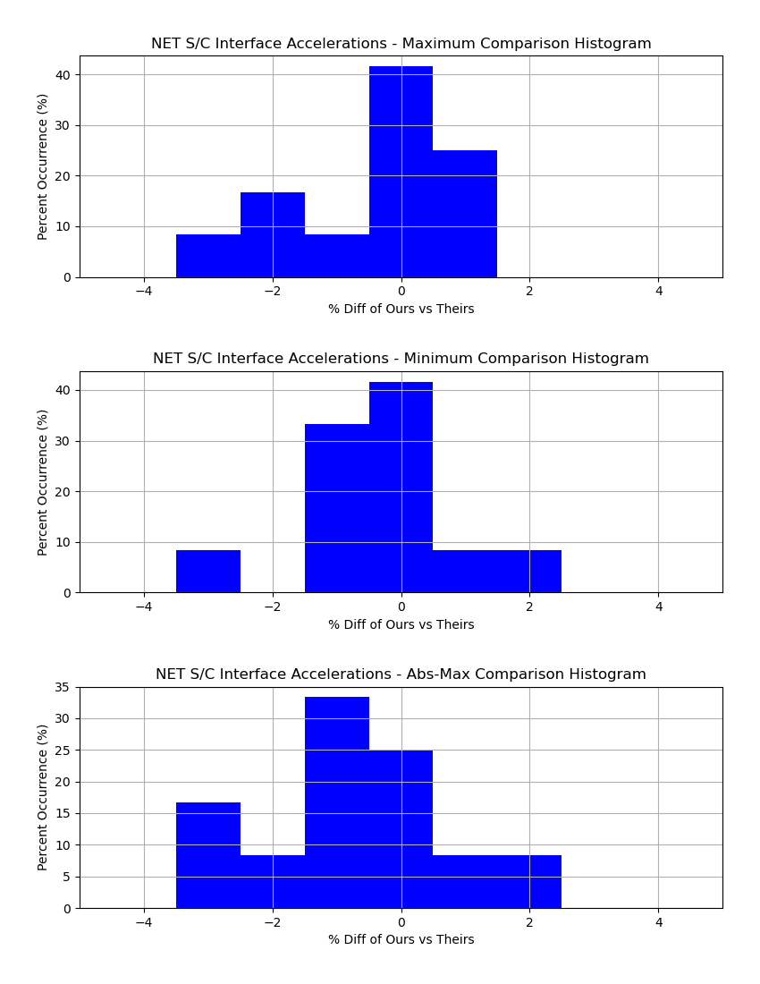
net_ifatm.cmp.histogram.png
Here is the “net_ifatm.cmp.magpct.png” file which is a scatter plot showing the comparisons of each data point versus the magnitude of “Theirs”. It uses the same color scheme as listed for the histogram data in a bar plot format. This plot gives a quick view of how the comparison looks over the range of small numbers to large numbers.

net_ifatm.cmp.magpct.png
Since the above “magpct” plot is not that interesting, here is the “scltm.cmp.magpct.png” file. The shaded out areas are for values smaller than the filter (which was left at the default +/- 1e-6 and shown by the dashed vertical lines), so our focus should be on the white, “Filtered region”. We can quickly see that there are values greater than 1000 that are off by more than 10%. More investigation would be needed to disposition these items. The specific rows can be determined from looking at the “scltm.cmp” file. In this case, all these differences were for CBAR bending moments and the only difference in the two sets of results is the version of Nastran used. (A deeper cause was not sought.)
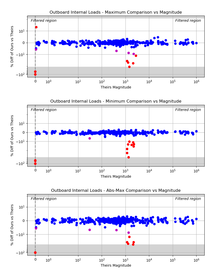
scltm.cmp.magpct.png