Fatigue damage equivalent PSDs

This and other notebooks are available here: https://github.com/twmacro/pyyeti/tree/master/docs/tutorials.

First, do some imports:

import numpy as np
import matplotlib.pyplot as plt
from pyyeti import psd, fdepsd
import scipy.signal as signal

Some settings specifically for the jupyter notebook.

%matplotlib inline
plt.rcParams['figure.figsize'] = [6.4, 4.8]
plt.rcParams['figure.dpi'] = 150.

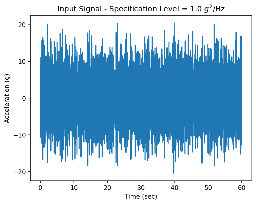
Generate a signal with flat content from 20 to 50 Hz

TF = 60  # make a 60 second signal
spec = np.array([[20, 1], [50, 1]])
sig, sr, t = psd.psd2time(spec, ppc=10, fstart=20,
                          fstop=50, df=1/TF,
                          winends=dict(portion=10),
                          gettime=True)
plt.plot(t, sig)
plt.title(r'Input Signal - Specification Level = '
           '1.0 $g^{2}$/Hz')
plt.xlabel('Time (sec)')
h = plt.ylabel('Acceleration (g)')

---

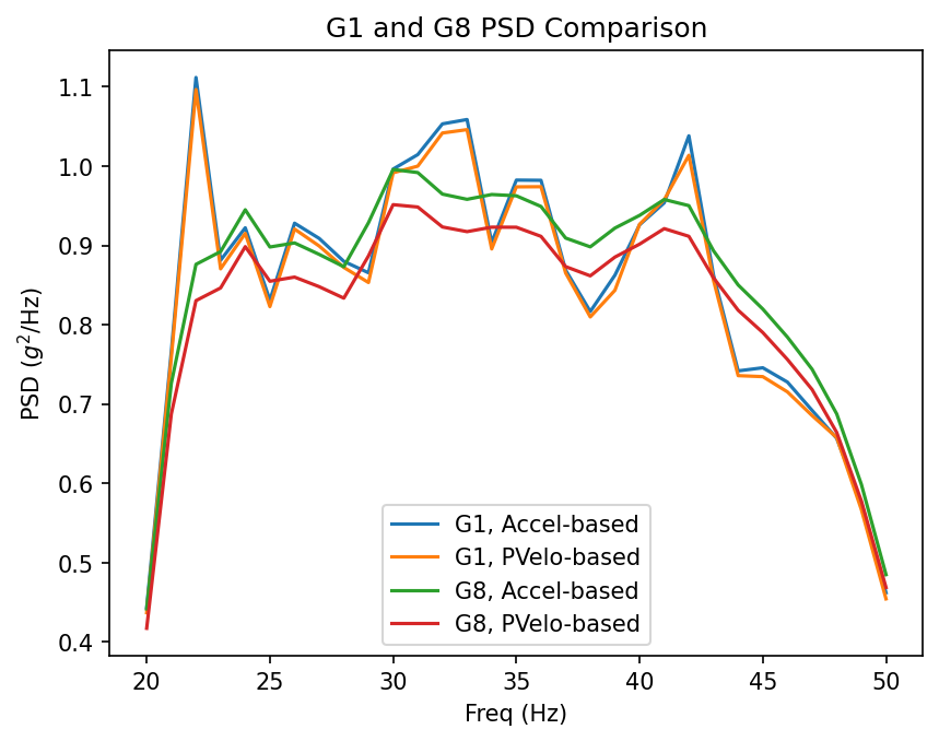
Compute fatigue damage equivalent PSDs using two different methods

One will use absolute-acceleration and the other will use pseudo-velocity. The plots will compare the G1 and G8 outputs. The output of the fdepsd function is a SimpleNamespace with several items; the main output is in the .psd member which has G1, G2, G4, G8 and G12 as columns in an array.

freq = np.arange(20., 50.1)
Q = 10
fde_acce = fdepsd.fdepsd(sig, sr, freq, Q)
fde_pvelo = fdepsd.fdepsd(sig, sr, freq, Q, resp='pvelo')

plt.plot(freq, fde_acce.psd['G1'], label='G1, Accel-based')
plt.plot(freq, fde_pvelo.psd['G1'], label='G1, PVelo-based')
plt.plot(freq, fde_acce.psd['G8'], label='G8, Accel-based')
plt.plot(freq, fde_pvelo.psd['G8'], label='G8, PVelo-based')
plt.title('G1 and G8 PSD Comparison')
plt.xlabel('Freq (Hz)')
plt.ylabel(r'PSD ($g^{2}$/Hz)')
h = plt.legend(loc='best')

---

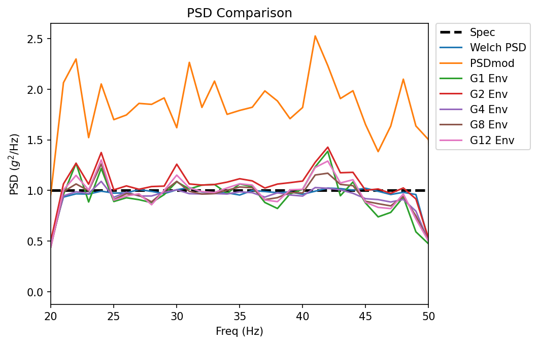
Compute fatigue damage equivalent PSDs to compare with standard PSDs

Form envelope over Q’s of 10, 25, 50.

psdenv = 0
freq = np.arange(20., 50.1)
for q in (10, 25, 50):
    fde = fdepsd.fdepsd(sig, sr, freq, q)
    psdenv = np.fmax(psdenv, fde.psd)

Compute standard Welch periodogram and use psd.psdmod for comparison

f, p = signal.welch(sig, sr, nperseg=sr)
f2, p2 = psd.psdmod(sig, sr, nperseg=sr, timeslice=4, tsoverlap=0.5)

Plot fatigue damage equivalents and the standard PSDs

spec = np.array(spec).T
plt.plot(*spec, 'k--', lw=2.5, label='Spec')
plt.plot(f, p, label='Welch PSD')
plt.plot(f2, p2, label='PSDmod')
psdenv.rename(
    columns={i: i + ' Env'
             for i in psdenv.columns}).plot.line(ax=plt.gca())
plt.xlim(20, 50)
plt.title('PSD Comparison')
plt.xlabel('Freq (Hz)')
plt.ylabel(r'PSD ($g^{2}$/Hz)')
h = plt.legend(loc='upper left',
               bbox_to_anchor=(1.02, 1.),
               borderaxespad=0.)

---

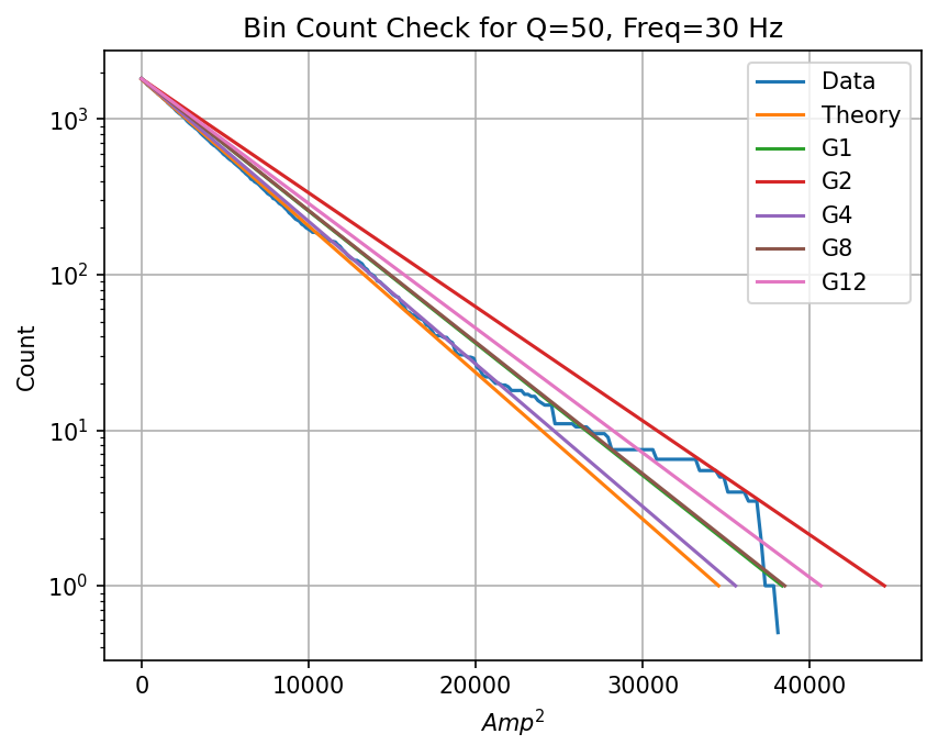
Compare cycle count results for 30 Hz to theoretical

This will be for Q = 50 since that was the last one run above.

Frq = freq[np.searchsorted(freq, 30)]

# First, plot counts vs. amplitude**2 from the data:
plt.semilogy(fde.binamps.loc[Frq]**2,
             fde.count.loc[Frq],
             label='Data')

# Compute theoretical curve: (use flight time here (TF),
# not test time (T0))

Amax2 = 2 * fde.var.loc[Frq] * np.log(Frq * TF)
plt.plot([0, Amax2], [Frq * TF, 1], label='Theory')

# Next, plot amp**2 vs total count for each PSD:
y1 = fde.count.loc[Frq, 0]
peakamp = fde.peakamp.loc[Frq]
for j, lbl in enumerate(fde.peakamp.columns):
    plt.plot([0, peakamp.iloc[j]**2], [y1, 1], label=lbl)
plt.title('Bin Count Check for Q=50, Freq=30 Hz')
plt.xlabel(r'$Amp^2$')
plt.ylabel('Count')
plt.grid(True)
h = plt.legend(loc='best')