Fatigue damage equivalent PSD

Tools for calculating the fatigue damage equivalent PSD. Adapted and enhanced from the CAM versions.

pyyeti.fdepsd.fdepsd(sig, sr, freq, Q, *, resp='absacce', detrend=True, winends='auto', hpfilter=5.0, nbins=300, T0=60.0, rolloff='lanczos', ppc=12, parallel='auto', maxcpu=14, verbose=False)

Compute a fatigue damage equivalent PSD from a signal.

Parameters:

• sig (1d array_like) – Base acceleration signal.

• sr (scalar) – Sample rate.

• freq (array_like) – Frequency vector in Hz. This defines the single DOF (SDOF) systems to use.

• Q (scalar > 0.5) – Dynamic amplification factor \(Q = 1/(2\zeta)\) where \(\zeta\) is the fraction of critical damping.

• resp (string; optional) – The type of response to base the damage calculations on:

  resp	Damage is based on
  ‘absacce’	absolute acceleration [1]
  ‘pvelo’	pseudo velocity [2]

• detrend (bool; optional) – If True, sig is detrended via scipy.signal.detrend(). Option is ignored and treated as True if at least one of the winends or hpfilter options are used. Detrending is done before either of those options.

• winends (None or ‘auto’ or dictionary; optional) – If None, pyyeti.dsp.windowends() is not called. If ‘auto’, pyyeti.dsp.windowends() is called to apply a 0.25 second window or a 50 point window (whichever is smaller) to the front. Otherwise, winends must be a dictionary of arguments that will be passed to pyyeti.dsp.windowends() (not including signal). The signal is detrended prior to calling pyyeti.dsp.windowends().

• hpfilter (scalar or None; optional) – High pass filter frequency; if None, no filtering is done. If filtering is done, it is after detrending and after any winends action was taken. The signal is filtered via scipy.signal.lfilter() using a 3rd order butterworth filter (scipy.signal.butter()).

• nbins (integer; optional) – The number of amplitude levels at which to count cycles

• T0 (scalar; optional) – Specifies test duration in seconds

• rolloff (string or function or None; optional) – Indicate which method to use to account for the SRS roll off when the minimum ppc value is not met. Either ‘fft’ or ‘lanczos’ seem the best. If a string, it must be one of these values:

  rolloff	Notes
  ‘fft’	Use FFT to upsample data as needed. See scipy.signal.resample().
  ‘lanczos’	Use Lanczos resampling to upsample as needed. See pyyeti.dsp.resample().
  ‘prefilter’	Apply a high freq. gain filter to account for the SRS roll-off. See pyyeti.srs.preroll() for more information. This option ignores ppc.
  ‘linear’	Use linear interpolation to increase the points per cycle (this is not recommended; method; it’s only here as a test case).
  ‘none’	Don’t do anything to enforce the minimum ppc. Note error bounds listed above.
  None	Same as ‘none’.

  If a function, the call signature is: sig_new, sr_new = rollfunc(sig, sr, ppc, frq). Here, sig is 1d, len(time). The last three inputs are scalars. For example, the ‘fft’ function is (trimmed of documentation):

  def fftroll(sig, sr, ppc, frq):
      N = sig.shape[0]
      if N > 1:
          curppc = sr/frq
          factor = int(np.ceil(ppc/curppc))
          sig = signal.resample(sig, factor*N, axis=0)
          sr *= factor
      return sig, sr
  

• ppc (scalar; optional) – Specifies the minimum points per cycle for SRS calculations. See also rolloff.

  ppc	Maximum error at highest frequency
  3	81.61%
  4	48.23%
  5	31.58%
  10	8.14% (minimum recommended ppc)
  12	5.67%
  15	3.64%
  20	2.05%
  25	1.31%
  50	0.33%

• parallel (string; optional) – Controls the parallelization of the calculations:

  parallel	Notes
  ‘auto’	Routine determines whether or not to run parallel.
  ‘no’	Do not use parallel processing.
  ‘yes’	Use parallel processing. Beware, depending on the particular problem, using parallel processing can be slower than not using it. On Windows, be sure the fdepsd() call is contained within: if __name__ == "__main__":
  ‘joblib’	Like ‘yes’ except use joblib for parallelization (see joblib.Parallel).

• maxcpu (integer or None; optional) – Specifies maximum number of CPUs to use. If None, it is internally set to 4/5 of available CPUs (as determined from multiprocessing.cpu_count()).

• verbose (bool or integer; optional) – If True (or > 0), routine will print some status information. If using joblib for parallelization, this value is passed as an integer to joblib.Parallel as well.

Returns:

• A SimpleNamespace with the members

• freq (1d ndarray) – Same as input freq.

• psd (pandas DataFrame; len(freq) x 5) – The amplitude and damage based PSDs. The index is freq and the five columns are: [G1, G2, G4, G8, G12]

  Name	Description
  G1	The “G1” PSD (Mile’s or similar equivalent from SRS); uses the maximum cycle amplitude instead of the raw SRS peak for each frequency. G1 is not a damage-based PSD.
  G2	The “G2” PSD of reference [1]; G2 >= G1 by bounding lower amplitude counts down to 1/3 of the maximum cycle amplitude. G2 is not a damage-based PSD.
  G4, G8, G12	The damage-based PSDs with fatigue exponents of 4, 8, and 12

• peakamp (pandas DataFrame; len(freq) x 5) – The peak response of SDOFs (single DOF oscillators) using each PSD as a base input. The index and the five columns are the same as for psd. The peaks are computed from the Mile’s equation (or similar if using resp='pvelo'). The peak factor used is sqrt(2*log(f*T0)). Note that the first column is, by definition, the maximum cycle amplitude for each SDOF from the rainflow count (G1 was calculated from this). Typically, this should be very close to the raw SRS peaks contained in the srs output but a little lower since SRS just grabs peaks without consideration of the opposite peak.

• binamps (pandas DataFrame; len(freq) x nbins) – A DataFrame of linearly spaced amplitude values defining the cycle counting bins. The index is freq and the columns are integers 0 to nbins - 1. The values in each row (for a specific frequency SDOF), range from 0.0 up to peakamp.loc[freq, "G1"] * (nbins - 1) / nbins. In other words, each value is the left-side amplitude boundary for that bin. The next column for this matrix would be peakamp.loc[:, "G1"].

• count (pandas DataFrame; len(freq) x nbins) – Summary matrix of the rainflow cycle counts. Size corresponds with binamps and the count is cumulative; that is, the count in each entry includes cycles at the binamps amplitude and above. Therefore, first column has total cycles for the SDOF.

• bincount (pandas DataFrame; len(freq) x nbins) – Non-cumulative version of count. In other words, the values are the number of cycles in the bin, left-side inclusive. The last bin includes the count of maximum amplitude cycles.

• di_sig (pandas DataFrame; len(freq) x 3) – Damage indicators computed from SDOF responses to the sig signal. Index is freq and columns are [‘b=4’, ‘b=8’, ‘b=12’]. The value for each frequency is the sum of the cycle count for a bin times its amplitude to the b power. That is, for the j-th frequency, the indicator is:

  amps = binamps.loc[freq[j]]
  counts = bincount.loc[freq[j]]
  
  di = (amps ** b) @ counts  # dot product of two vectors
  

  Note that this definition is slightly different than equation 14 from [1] (would have to divide by the frequency), but the same as equation 10 of [2] without the constant.

• di_test_part (pandas DataFrame; len(freq) x 3) – Test damage indicator without including the variance factor (see note). Same size as di_sig. Each value depends only on the frequency, T0, and the fatigue exponent b. The ratio of a signal damage indicator to the corresponding partial test damage indicator is equal to the variance of the single DOF response to the test raised to the b / 2 power:

  var_test ** (b / 2) = di_sig / di_test_part
  

  Note

  If the variance factor (var_test) were included, then the test damage indicator would be the same as di_sig. This relationship is the basis of determining the amplitude of the test signal.

• var_test (pandas DataFrame; len(freq) x 3) – The required SDOF test response variances (see di_test_part description). Same size as di_sig. The amplitude of the G4, G8, and G12 columns of psd are computed from Mile’s equation (or similar) and var_test.

• sig (1d ndarray) – The version of the input sig that is fed into the fatique damage algorithm. This would be after any filtering, windowing, and upsampling.

• sr (scalar) – The sample rate of the output sig.

• srs (pandas Series; length = len(freq)) – The raw SRS peaks version of the first column in amp. See amp. Index is freq.

• var (pandas Series; length = len(freq)) – Vector of the SDOF response variances. Index is freq.

• parallel (string) – Either ‘yes’ or ‘no’ depending on whether parallel processing was used or not.

• ncpu (integer) – Specifies the number of CPUs used.

• resp (string) – Same as the input resp.

• use_joblib (bool) – True if joblib was used for parallelization.

Notes

Steps (see [1], [2]):

1. Resample signal to higher rate if highest frequency would have less than ppc points-per-cycle. Method of increasing the sample rate is controlled by the rolloff input.

2. For each frequency:

   1. Compute the SDOF base-drive response

   2. Calculate srs and var outputs

   3. Use pyyeti.cyclecount.findap() to find cycle peaks

   4. Use pyyeti.cyclecount.rainflow() to count cycles and amplitudes

   5. Put counts into amplitude bins

3. Calculate g1 based on cycle amplitudes from maximum amplitude (step 2d) and Mile’s (or similar) equation.

4. Calculate g2 to bound g1 & lower amplitude cycles with high counts. Ignore amplitudes < Amax/3.

5. Calculate damage indicators from data with b = 4, 8, 12 where b is the fatigue exponent.

6. By equating the theoretical damage from a T0 second random vibration test to the damage from the input signal (step 5), solve for the required test response variances for b = 4, 8, 12.

7. Solve for g4, g8, g12 from the results of step 6 using the Mile’s equation (or similar); equations are shown below.

No checks are done regarding the suitability of this method for the input data. It is recommended to read the references [1] [2] and do those checks (such as plotting Count or Time vs. Amp**2 and comparing to theoretical).

The Mile’s equation (or similar) is used in this methodology to relate acceleration PSDs to peak responses. If resp is ‘absacce’, it is the Mile’s equation:

\[\sigma_{absacce}(f) = \sqrt{\frac{\pi}{2} \cdot f \cdot Q \cdot PSD(f)}\]

If resp is ‘pvelo’, the similar equation is:

\[\sigma_{pvelo}(f) = \sqrt{\frac{Q \cdot PSD(f)}{8 \pi f}}\]

Those two equations assume a flat acceleration PSD. Therefore, it is recommended to compare SDOF responses from flight data (SRS) to SDOF VRS responses from the developed specification (see pyyeti.srs.vrs() to compute the VRS response in the absolute-acceleration case). This is to check for conservatism. Instead of using 3 for peak factor (for 3-rms or 3-sigma), use \(\sqrt{2 \ln(f \cdot T_0)}\) for the peak factor (derived below). Also, enveloping multiple specifications from multiple Q’s is worth considering.

Note that this analysis can be time consuming; the time is proportional to the number of frequencies multiplied by the number of time steps in the signal.

The derivation of the peak factor is as follows. For the special case of narrow band noise where the instantaneous amplitudes follow the Gaussian distribution, the resulting probability density function for the peak amplitudes follow the Rayleigh distribution [3]. The single DOF response to Gaussian input is reasonably estimated as Gaussian narrow band. Let this response have the standard deviation \(\sigma\). From the Rayleigh distribution, the probability of a peak being greater than \(A\) is:

\[Prob[peak > A] = e ^ {\frac{-A^2}{2 \sigma^2}}\]

To estimate the maximum peak for the response of a single DOF system with frequency \(f\), find the amplitude that would be expected to occur once within the allotted time (\(T_0\)). That is, set the product of the probability of a cycle amplitude being greater than \(A\) and the number of cycles equal to 1.0, and then solve for \(A\).

The number of cycles of \(f\) Hz is \(N = f \cdot T_0\).

Therefore:

\[ \begin{align}\begin{aligned}\begin{aligned}\\Prob[peak > A] \cdot N &= 1.0\\e ^ {\frac{-A^2}{2 \sigma^2}} f \cdot T_0 &= 1.0\\\frac{-A^2}{2 \sigma^2} &= \ln(1.0) - \ln(f \cdot T_0)\\\frac{A^2}{2 \sigma^2} &= \ln(f \cdot T_0)\\A &= \sqrt{2 \ln(f \cdot T_0)} \sigma\\\end{aligned}\end{aligned}\end{align} \]

Note

In addition to the example shown below, this routine is demonstrated in the pyYeti Tutorials: Fatigue damage equivalent PSDs. There is also a link to the source Jupyter notebook at the top of the tutorial.

References

[1] (1,2,3,4,5)

“Analysis of Nonstationary Vibroacoustic Flight Data Using a Damage-Potential Basis”; S. J. DiMaggio, B. H. Sako, S. Rubin; Journal of Spacecraft and Rockets, Vol 40, No. 5, September-October 2003.

[2] (1,2,3,4)

“Implementing the Fatigue Damage Spectrum and Fatigue Damage Equivalent Vibration Testing”; Scot I. McNeill; 79th Shock and Vibration Symposium, October 26 – 30, 2008.

[3]

Bendat, Julius S., “Probability Functions for Random Responses: Prediction of Peaks, Fatigue Damage, and Catastrophic Failures”, NASA Contractor Report 33 (NASA CR-33), 1964.

See also

scipy.signal.welch(), pyyeti.psd.psdmod(), pyyeti.cyclecount.rainflow(), pyyeti.srs.srs()

Examples

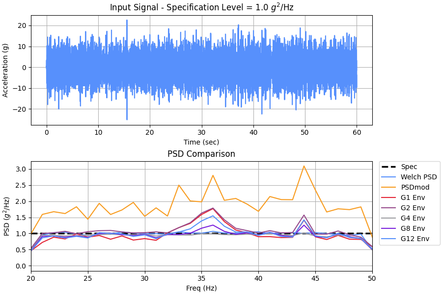
Generate 60 second random signal to a pre-defined spec level, compute the PSD several different ways and compare. Since it’s 60 seconds, the damage-based PSDs should be fairly close to the input spec level. The damage-based PSDs will be calculated with several Qs and enveloped.

In this example, G2 envelopes G1, G4, G8, G12. This is not always the case. For example, try TF=120; the damage-based curves go up in order to fit equal damage in 60s.

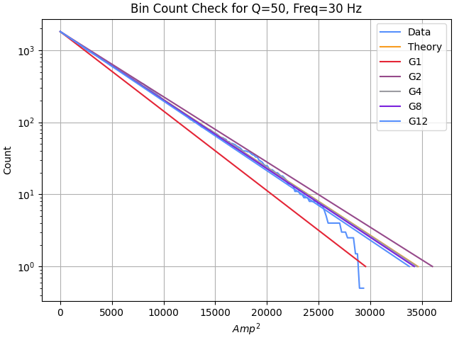
One Count vs. Amp**2 plot is done for illustration.

>>> import numpy as np
>>> import matplotlib.pyplot as plt
>>> from pyyeti import psd, fdepsd
>>> import scipy.signal as signal
>>>
>>> TF = 60  # make a 60 second signal
>>> spec = np.array([[20, 1], [50, 1]])
>>> sig, sr, t = psd.psd2time(
...     spec, ppc=10, fstart=20, fstop=50, df=1 / TF,
...     winends=dict(portion=10), gettime=True)
>>>
>>> fig = plt.figure('Example', figsize=[9, 6], clear=True,
...                  layout='constrained')
>>> _ = plt.subplot(211)
>>> _ = plt.plot(t, sig)
>>> _ = plt.title(r'Input Signal - Specification Level = '
...               '1.0 $g^{2}$/Hz')
>>> _ = plt.xlabel('Time (sec)')
>>> _ = plt.ylabel('Acceleration (g)')
>>> ax = plt.subplot(212)
>>> f, p = signal.welch(sig, sr, nperseg=sr)
>>> f2, p2 = psd.psdmod(sig, sr, nperseg=sr, timeslice=4,
...                     tsoverlap=0.5)

Calculate G1, G2, and the damage potential PSDs:

>>> psd_ = 0
>>> freq = np.arange(20., 50.1)
>>> for q in (10, 25, 50):
...     fde = fdepsd.fdepsd(sig, sr, freq, q)
...     psd_ = np.fmax(psd_, fde.psd)
>>> #
>>> _ = plt.plot(*spec.T, 'k--', lw=2.5, label='Spec')
>>> _ = plt.plot(f, p, label='Welch PSD')
>>> _ = plt.plot(f2, p2, label='PSDmod')
>>>
>>> # For plot, rename columns in DataFrame to include "Env":
>>> psd_ = (psd_
...         .rename(columns={i: i + ' Env'
...                          for i in psd_.columns}))
>>> _ = psd_.plot.line(ax=ax)
>>> _ = plt.xlim(20, 50)
>>> _ = plt.title('PSD Comparison')
>>> _ = plt.xlabel('Freq (Hz)')
>>> _ = plt.ylabel(r'PSD ($g^{2}$/Hz)')
>>> _ = plt.legend(loc='upper left',
...                bbox_to_anchor=(1.02, 1.),
...                borderaxespad=0.)

Compare to theoretical bin counts @ 30 Hz:

>>> _ = plt.figure('Example 2', clear=True,
...                layout='constrained')
>>> Frq = freq[np.searchsorted(freq, 30)]
>>> _ = plt.semilogy(fde.binamps.loc[Frq]**2,
...                  fde.count.loc[Frq],
...                  label='Data')
>>> # use flight time here (TF), not test time (T0)
>>> Amax2 = 2 * fde.var.loc[Frq] * np.log(Frq * TF)
>>> _ = plt.plot([0, Amax2], [Frq * TF, 1], label='Theory')
>>> y1 = fde.count.loc[Frq, 0]
>>> peakamp = fde.peakamp.loc[Frq]
>>> for j, lbl in enumerate(fde.peakamp.columns):
...     _ = plt.plot(
...         [0, peakamp.iloc[j]**2], [y1, 1], label=lbl
...     )
>>> _ = plt.title('Bin Count Check for Q=50, Freq=30 Hz')
>>> _ = plt.xlabel(r'$Amp^2$')
>>> _ = plt.ylabel('Count')
>>> _ = plt.legend(loc='best')