pyyeti.frclim.ntfl
- pyyeti.frclim.ntfl(Source, Load, As, freq)[source]
Norton-Thevenin Force Limit
- Parameters:
Source (list/tuple or 3d ndarray) –
Can be either:
list/tuple of
[mass, damp, stiff, bdof]for Source (eg, launch vehicle). These are the Source mass, damping, and stiffness matrices (seepyyeti.ode.SolveUnc) and bdof, which is described below.SAM, a 3d ndarray of Source apparent mass (from a previous run). See description of outputs.
Load (list/tuple or 3d ndarray) – Same format as Source except for the “Load” (eg, spacecraft)
As (2d array_like) – Free-acceleration of the Source (interface acceleration without the Load attached).
freq (1d array_like) – Frequency vector in Hz for Source, Load, As and all return values.
- Returns:
A SimpleNamespace with the members
A (2d ndarray) – Coupled system interface acceleration, complex, # bdof x len(freq).
F (2d ndarray) – Coupled system interface force, complex, # bdof x len(freq)
R (2d ndarray) – Norton-Thevenin normalized response ratio; complex, # bdof x len(freq). R is independent of As. Each row of R is the diagonal of the ratio of the loaded-response over the free-response, which is the same as the diagonal of the Source apparent mass over the Total apparent mass.
LAM, SAM, TAM (3d ndarrays) – Load, Source and Total apparent mass matrices:
boundary DOF x Frequencies x boundary DOF
 (response)                   (input)
TAM = SAM + LAMfreq (1d array_like) – Copy of the input freq.
Notes
The Norton-Thevenin (NT) equations couple the Source and Load models together in an exact way in the frequency domain. It is a very convenient formulation for force-limiting applications simply because the Source and Load models are kept separate and coupled system responses are computed by using the “apparent mass” of both models and the “free-acceleration” of the Source. If those quantities are known exactly, the responses computed from the NT equations are also exact.
Apparent Mass
The term “apparent mass” is very apt. Apparent mass is also known as “dynamic mass”, and its inverse is known as “inertance” or “accelerance”. If you were to grab some point on a structure and push and pull in a sinusoidal fashion at some frequency, the amount of mass you would feel resisting you is the apparent mass. It varies by frequency. At zero Hz (for rigid-body motion), there is no vibration and the mass you feel is the physical mass of the structure. At frequencies greater than zero, the structure will vibrate and “inertial forces” (mass x acceleration) will come into play. Inertial forces can either push against you – so apparent mass > physical mass – or work with you – so apparent mass < physical mass.
To compute the apparent mass for the Source (or the Load) relative to the boundary “b” DOF that attach to the Load (or the Source), consider this frequency domain equation:
\[\ddot{X}_{b}(\Omega) = H_{bb}(\Omega) \cdot F_{b}(\Omega)\]The transfer function \(H_{bb}(\Omega)\) is known as “inertance” or “accelerance”. By applying unit forces to the “b” DOF one at a time (so that \(F_{b}(\Omega)\) is identity), the response \(\ddot{X}_{b}(\Omega)\) is equal to \(H_{bb}(\Omega)\). The apparent mass \(AM_{bb}(\Omega)\) is simply the inverse of the accelerance \(H_{bb}(\Omega)\):
\[\begin{split}\begin{array}{c} AM_{bb}(\Omega) = {H_{bb}(\Omega)}^{-1} \\ F_{b} (\Omega) = AM_{bb}(\Omega) \cdot \ddot{X}_{b}(\Omega) \end{array}\end{split}\]This is Newton’s second law (
F = ma) in the frequency domain. The routinecalcAM()calculates the apparent mass.Free-Acceleration
The term “free-acceleration” is also quite apt. With all Source external forces applied as normal, “free-acceleration” is the acceleration response of the Source “b” DOF with those DOF in a free-free boundary condition (that is, without the Load attached).
Deriving the NT Coupling Equations
Consider the equations of motion for the Source (“S”) or the Load (“L”):
\[\begin{split}\left\{ \begin{array}{c} \ddot{X}_b(\Omega) \\ \ddot{X}_o(\Omega) \end{array} \right\}_{S~or~L} = \left[ \begin{array}{cc} H_{bb}(\Omega) & H_{bo}(\Omega) \\ H_{ob}(\Omega) & H_{oo}(\Omega) \end{array} \right]_{S~or~L} \left\{ \begin{array}{c} F_b(\Omega) + \tilde{F}_b(\Omega) \\ F_o(\Omega) \end{array} \right\}_{S~or~L}~~~~~~~(1)\end{split}\]Here, the “o” DOF are all other DOF (DOF that are not on the boundary), \(F_b\) and \(F_o\) are externally applied forces, and \(\tilde{F}_b\) are forces from the other component.
For joint compatibility, we need equal accelerations, and equal but opposite forces:
\[\begin{split}\begin{array}{c} \ddot{X}_{b,L}(\Omega) = \ddot{X}_{b,S}(\Omega) = \ddot{X}_b(\Omega) \\ \tilde{F}_{b,L}(\Omega) = - \tilde{F}_{b,S}(\Omega) = \tilde{F}_b(\Omega) \end{array}\end{split}\]For the Load without any externally applied forces, \(F_{b,L} = 0\) and \(F_{o,L} = 0\), the 1st partition of equation (1) becomes:
\[\ddot{X}_b(\Omega) = H_{bb,L}(\Omega) \cdot \tilde{F}_b(\Omega)\]Or:
\[\tilde{F}_b(\Omega) = AM_{bb,L}(\Omega) \cdot \ddot{X}_b(\Omega)~~~~~~~(2)\]To derive an equation for the free-acceleration \(A_S(\Omega)\), set \(\tilde{F}_{b,S} \rightarrow 0\) (since there is no Load attached) in equation (1):
\[A_S(\Omega) = \ddot{X}_{b,S,no-Load}(\Omega) = H_{bb,S}(\Omega) \cdot F_{b,S}(\Omega) + H_{bo,S}(\Omega) \cdot F_{o,S}(\Omega)\]Therefore, the top of equation (1) for the Source can be written as (remembering that \(\tilde{F}_{b,S}(\Omega) = - \tilde{F}_b(\Omega)\)):
\[\ddot{X}_b(\Omega) = - H_{bb,S}(\Omega) \cdot \tilde{F}_{b}(\Omega) + A_S(\Omega)~~~~~~~(3)\]Substituting equation (2) into (3) and collecting terms:
\[\begin{split}\begin{array}{c} \ddot{X}_b(\Omega) = - H_{bb,S}(\Omega) \cdot AM_{bb,L}(\Omega) \cdot \ddot{X}_b(\Omega) + A_S(\Omega) \\ (I + H_{bb,S}(\Omega) \cdot AM_{bb,L}(\Omega)) \cdot \ddot{X}_b(\Omega) = A_S(\Omega) \end{array}\end{split}\]Multiplying that result by the Source apparent mass gives:
\[(AM_{bb,S}(\Omega) + AM_{bb,L}(\Omega)) \cdot \ddot{X}_b(\Omega) = AM_{bb,S}(\Omega) \cdot A_S(\Omega)\]Solving for \(\ddot{X}_b(\Omega)\):
\[\ddot{X}_b(\Omega) = (AM_{bb,S}(\Omega) + AM_{bb,L}(\Omega))^{-1} \cdot AM_{bb,S}(\Omega) \cdot A_S(\Omega)~~~~~~~(4)\]After solving for \(\ddot{X}_b(\Omega)\) from equation (4), we can solve for \(\tilde{F}_b(\Omega)\) from equation (2). We can also use equation (4) to expand equation (2):
\[\tilde{F}_b(\Omega) = AM_{bb,L}(\Omega) \cdot (AM_{bb,S}(\Omega) + AM_{bb,L}(\Omega))^{-1} \cdot AM_{bb,S}(\Omega) \cdot A_S(\Omega)~~~~~~~(5)\]Outputs of this routine
The outputs are computed as follows:
\[\begin{split}\begin{aligned} A(\Omega) &= \ddot{X}_b(\Omega) = (AM_{bb,S}(\Omega) + AM_{bb,L}(\Omega))^{-1} \cdot AM_{bb,S}(\Omega) \cdot A_S(\Omega) \\ F(\Omega) &= \tilde{F}_b(\Omega) = AM_{bb,L}(\Omega) \cdot A(\Omega) \\ R(\Omega) &= diag((AM_{bb,S}(\Omega) + AM_{bb,L}(\Omega))^{-1} \cdot AM_{bb,S}(\Omega)) \\ \end{aligned}\end{split}\]On output, the 3D apparent mass arrays are named as follows:
\[\begin{split}\begin{aligned} AM_{bb,L}(\Omega) & \rightarrow LAM \\ AM_{bb,S}(\Omega) & \rightarrow SAM \\ AM_{bb,L}(\Omega) + AM_{bb,S}(\Omega) & \rightarrow TAM \end{aligned}\end{split}\]The bdof input defines boundary DOF in one of two ways as follows. Let N be total number of DOF in mass, damping, & stiffness.
If bdof is a 2d array_like, it is interpreted to be a data recovery matrix to the b-set (number b-set =
bdof.shape[0]). Structure is treated generically (usespyyeti.ode.SolveUncwithpre_eig=Trueto compute apparent mass).Otherwise, bdof is assumed to be a 1d partition vector from full N size to b-set and structure is assumed to be in Craig-Bampton form (uses
pyyeti.cb.cbtf()to compute apparent mass).
Note that the Source and Load bdof must define the same number of boundary DOF and both sets of boundary DOF must be in the same coordinate system.
Tips
If using a free-free model, include residual vectors defined relative to the boundary DOF. These can be critical for retaining the boundary flexibility needed for accurate results even in the lowest system frequencies. This is because boundary stiffness that only participates in very high frequency modes with a free-free boundary condition can participate in the lowest frequency modes when connected to another model.
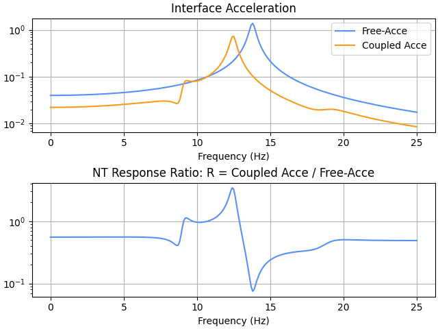
The free-acceleration of the Source is the complex response of the boundary DOF without the Load attached. Frequency domain envelopes of flight data, or vibration specifications derived from envelopes, are not accurate ways to come up with the free-acceleration because a Load is attached. However, since this is sometimes the only viable option, is it conservative? Conservatism becomes more and more likely with this approach as the number of enveloped curves increases. This is because, for a given Load, the coupled system response will likely exceed the free-acceleration response in some frequency bands. See, for example, the final two subplots in the example below; the coupled system response is higher than the free-acceleration response at 12.5 Hz. Such enveloping can therefore lead to a very conservative free-acceleration curve, which means conservative results.
As was noted, coupled system responses can exceed free-acceleration in some frequency bands (for example, at 12.5 Hz in the system demonstrated below). This means that, in cases where a bounding coupled system acceleration level is used for the free-acceleration, application of the NT equations will likely result in responses that exceed the bound. To avoid excessive conservatism, it may be prudent in these cases to accept any notching down, but to not allow “notching up”. That is; do not let \(A(\Omega)\) exceed \(As(\Omega)\).
The apparent mass of a structure can be used to perform frequency domain base-drive analyses instead of using a seismic mass. Just compute the force required to meet the acceleration requirement via equation (2) above (\(\tilde{F}_b(\Omega) = AM_{bb}(\Omega) \cdot \ddot{X}_b(\Omega)\)). Note that a simple matrix multiply will not work for all frequencies at the same time since the apparent mass is a 3D array. You could use a loop, or you could use the remarkable
numpy.einsum()function:F = numpy.einsum('ijk,kj->ij', AM, Xdd)
Notional example:
from pyyeti import frclim
from pyyeti.nastran op2, n2p, op4
import pickle

# load free-acceleration of LV
dct = pickle.load('ifresults_free.p')
As = dct['As']
freq = dct['freq']

# load Source free-free model, with residual vectors included
nas = op2.rdnas2cam('nas2cam')
m1 = None
zeta = 0.01
k1 = nas['lambda'][0]
k1[:nas['nrb']] = 0.
b1 = 2*zeta*np.sqrt(k1)

# Transformation to i/f node:
T, dof = n2p.formdrm(nas, seup=0, sedn=0, dof=888888)

# get S/C mass and stiffness of Load:
mk = op4.read('mk.op4')
kgen = mk['kgen']
mgen = mk['mgen']
kgen[:6, :6] = 0.
zeta = 0.01
bgen = np.diag(2*zeta*np.sqrt(np.diag(kgen)))

# Norton-Thevenin force limit function:
r = frclim.ntfl([m1, b1, k1, T], [mgen, bgen, kgen,
                np.arange(6)], As, freq)
Note
In addition to the example shown below, this routine is demonstrated in the pyYeti Tutorials: Coupling models together using the Norton-Thevenin method. There is also a link to the source Jupyter notebook at the top of the tutorial.
Examples
This example sets up a simple mass-spring system to demonstrate that the Norton-Thevenin equations can be exact.
Steps:
Setup a coupled system of a SOURCE and a LOAD
Solve for interface acceleration and force from coupled system (frequency domain)
Calculate free-acceleration from SOURCE alone and setup LOAD
Use
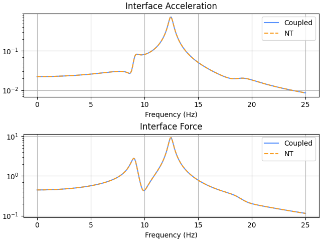
ntfl()to couple the systemPlot interface acceleration and force to show
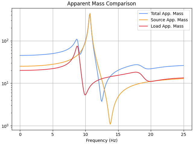
ntfl()can be an exact coupling methodPlot apparent masses
Plot free-acceleration and coupled acceleration
Plot normalized response ratio (can be thought of as force limiting factor)
Setup system:
        |--> x1       |--> x2        |--> x3        |--> x4
        |             |              |              |
     |----|    k1   |----|    k2   |----|    k3   |----|
 Fe  |    |--\/\/\--|    |--\/\/\--|    |--\/\/\--|    |
====>| 10 |         | 30 |         |  3 |         |  2 |
     |    |---| |---|    |---| |---|    |---| |---|    |
     |----|    c1   |----|    c2   |----|    c3   |----|

     |<--- SOURCE --->||<------------ LOAD ----------->|
Define parameters:
>>> import numpy as np
>>> from pyyeti import frclim, ode
>>> freq = np.arange(0.0, 25.1, 0.1)
>>> M1 = 10.
>>> M2 = 30.
>>> M3 = 3.
>>> M4 = 2.
>>> c1 = 15.
>>> c2 = 15.
>>> c3 = 15.
>>> k1 = 45000.
>>> k2 = 25000.
>>> k3 = 10000.
Solve coupled system:
>>> MASS = np.array([[M1, 0, 0, 0],
...                  [0, M2, 0, 0],
...                  [0, 0, M3, 0],
...                  [0, 0, 0, M4]])
>>> DAMP = np.array([[c1, -c1, 0, 0],
...                  [-c1, c1+c2, -c2, 0],
...                  [0, -c2, c2+c3, -c3],
...                  [0, 0, -c3, c3]])
>>> STIF = np.array([[k1, -k1, 0, 0],
...                  [-k1, k1+k2, -k2, 0],
...                  [0, -k2, k2+k3, -k3],
...                  [0, 0, -k3, k3]])
>>> F = np.vstack((np.ones((1, len(freq))),
...                np.zeros((3, len(freq)))))
>>> fs = ode.SolveUnc(MASS, DAMP, STIF, pre_eig=True)
>>> fullsol = fs.fsolve(F, freq)
>>> A_coupled = fullsol.a[1]
>>> F_coupled = (M2/2*A_coupled -
...              k2*(fullsol.d[2] - fullsol.d[1]) -
...              c2*(fullsol.v[2] - fullsol.v[1]))
Solve for free-acceleration; SOURCE setup: [m, b, k, bdof]:
>>> ms = np.array([[M1, 0], [0, M2/2]])
>>> cs = np.array([[c1, -c1], [-c1, c1]])
>>> ks = np.array([[k1, -k1], [-k1, k1]])
>>> source = [ms, cs, ks, [[0, 1]]]
>>> fs_source = ode.SolveUnc(ms, cs, ks, pre_eig=True)
>>> sourcesol = fs_source.fsolve(F[:2], freq)
>>> As = sourcesol.a[1:2]   # free-acceleration
LOAD setup: [m, b, k, bdof]:
>>> ml = np.array([[M2/2, 0, 0], [0, M3, 0], [0, 0, M4]])
>>> cl = np.array([[c2, -c2, 0], [-c2, c2+c3, -c3], [0, -c3, c3]])
>>> kl = np.array([[k2, -k2, 0], [-k2, k2+k3, -k3], [0, -k3, k3]])
>>> load = [ml, cl, kl, [[1, 0, 0]]]
4. Use NT to couple equations. First value (rigid-body motion) should equal
Source Mass / Total Mass = 25/45 = 0.55555...Results should match the coupled method.>>> r = frclim.ntfl(source, load, As, freq) >>> abs(r.R[0, 0]) 0.55555... >>> np.allclose(A_coupled, r.A) True >>> np.allclose(F_coupled, r.F) True
Calculate the total apparent mass directly using
calcAM(). This should match ther.TAMvalue.>>> TAM = frclim.calcAM((MASS, DAMP, STIF, [[0, 1, 0, 0]]), freq) >>> np.allclose(TAM, r.TAM) True >>> np.allclose(TAM, r.SAM+r.LAM) True
Plot comparisons:
>>> import matplotlib.pyplot as plt
>>> _ = plt.figure('Example', clear=True, layout='constrained')
>>> _ = plt.subplot(211)
>>> _ = plt.semilogy(freq, abs(A_coupled),
...                  label='Coupled')
>>> _ = plt.semilogy(freq, abs(r.A).T, '--',
...                  label='NT')
>>> _ = plt.title('Interface Acceleration')
>>> _ = plt.xlabel('Frequency (Hz)')
>>> _ = plt.legend(loc='best')
>>> _ = plt.subplot(212)
>>> _ = plt.semilogy(freq, abs(F_coupled),
...                  label='Coupled')
>>> _ = plt.semilogy(freq, abs(r.F).T, '--',
...                  label='NT')
>>> _ = plt.title('Interface Force')
>>> _ = plt.xlabel('Frequency (Hz)')
>>> _ = plt.legend(loc='best')
Plot apparent masses:
>>> _ = plt.figure('Example 2', clear=True,
...                layout='constrained')
>>> _ = plt.semilogy(freq, abs(r.TAM[0, :, 0]),
...                  label='Total App. Mass')
>>> _ = plt.semilogy(freq, abs(r.SAM[0, :, 0]),
...                  label='Source App. Mass')
>>> _ = plt.semilogy(freq, abs(r.LAM[0, :, 0]),
...                  label='Load App. Mass')
>>> _ = plt.title('Apparent Mass Comparison')
>>> _ = plt.xlabel('Frequency (Hz)')
>>> _ = plt.legend(loc='best')
Plot accelerations and
Plot force limit factor:
>>> _ = plt.figure('Example 3', clear=True,
...                layout='constrained')
>>> _ = plt.subplot(211)
>>> _ = plt.semilogy(freq, abs(As).T,
...                  label='Free-Acce')
>>> _ = plt.semilogy(freq, abs(r.A).T,
...                  label='Coupled Acce')
>>> _ = plt.title('Interface Acceleration')
>>> _ = plt.xlabel('Frequency (Hz)')
>>> _ = plt.legend(loc='best')
>>> _ = plt.subplot(212)
>>> _ = plt.semilogy(freq, abs(r.R).T)
>>> _ = plt.title('NT Response Ratio: '
...               'R = Coupled Acce / Free-Acce')
>>> _ = plt.xlabel('Frequency (Hz)')