pyyeti.frclim.calcAM

pyyeti.frclim.calcAM(S, freq, fs=None)

Calculate apparent mass

Apparent mass is also known as “dynamic mass”. The inverse of apparent mass is known as “inertance” or “accelerance”. See ntfl() for more discussion.

Parameters:

• S (list/tuple) – Contains: [mass, damp, stiff, bdof] for structure. These are the Source mass, damping, and stiffness matrices (see pyyeti.ode.SolveUnc) and bdof, which is described below.

• freq (1d array_like) – Frequency vector (Hz)

• fs (class instance or None; optional) – If None, this routine will try pyyeti.ode.SolveUnc with pre_eig=True to solve equations of motion in frequency domain. If pyyeti.ode.SolveUnc fails, this routine will then try pyyeti.ode.FreqDirect. If fs is not None, it is excpected to be an instance of pyyeti.ode.SolveUnc or pyyeti.ode.FreqDirect (or similar … must have .fsolve method)

  Note

  Using the fs parameter is the only way to include residual vectors statically with this routine.

  Note

  The fs parameter is ignored if bdof is 1d; the pyyeti.cb.cbtf() routine is used to compute apparent mass in that case (see Notes below).

Returns:

AM (3d ndarray) – Apparent mass matrix in a 3d array:

boundary DOF x Frequencies x boundary DOF
 (response)                   (input)

Notes

The bdof input defines boundary DOF in one of two ways as follows. Let N be total number of DOF in mass, damping, & stiffness.

1. If bdof is a 2d array_like, it is interpreted to be a data recovery matrix to the b-set (number b-set = bdof.shape[0]). Structure is treated generically (uses pyyeti.ode.SolveUnc with pre_eig=True to compute apparent mass).

2. Otherwise, bdof is assumed to be a 1d partition vector from full N size to b-set and structure is assumed to be in Craig-Bampton form (uses pyyeti.cb.cbtf() to compute apparent mass).

Note

In addition to the example shown below, this routine is demonstrated in the pyYeti Tutorials: Coupling models together using the Norton-Thevenin method. There is also a link to the source Jupyter notebook at the top of the tutorial.

See also

ntfl()

Examples

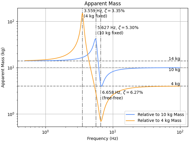
Consider the 2 DOF system:

|----|    k    |----|
|    |--\/\/\--|    |
| m1 |         | m2 |
|    |---| |---|    |
|----|    c    |----|

Where:

    m1 = 10.0 kg
    m2 = 4.0 kg
    k = 5000.0 N/m
    c = 15.0 N/(m/s)

The following will plot the apparent mass curves relative to each of the masses, and annotate the plot with three mass values (4, 10, & 14 kg) and three frequency values (free-free, with the 4 kg mass fixed, and with the 10 kg mass fixed). The percent critical damping ratio is also included for each of the three boundary conditions. The annotations are meant as an aide to guide intuition.

>>> import numpy as np
>>> from scipy.linalg import eigh
>>> import matplotlib.pyplot as plt
>>> from pyyeti import frclim
>>>
>>> m1 = 10.0
>>> m2 = 4.0
>>> k = 5000.0
>>> c = 15.0
>>>
>>> M = np.diag([m1, m2])
>>> K = np.array([[k, -k], [-k, k]])
>>> C = np.array([[c, -c], [-c, c]])
>>>
>>> # compute free-free frequencies (1st is 0 Hz rigid-body mode)
>>> lam_ff, phi_ff = eigh(K, M)
>>> omega_ff = np.sqrt(abs(lam_ff))
>>> frq_ff = omega_ff / 2 / np.pi
>>>
>>> C_ff = phi_ff.T @ C @ phi_ff
>>> zeta_ff = C_ff[1, 1] / 2 / omega_ff[1]
>>>
>>> freq = np.geomspace(0.5, 100.0, 500)
>>> fig = plt.figure("apparent mass", clear=True,
...                  layout='constrained')
>>> ax = fig.subplots(1, 1)
>>>
>>> fx_frqs = []
>>> fx_zetas = []
>>> for fixed, lbl in (
...     (np.array([True, False]), "Relative to 10 kg Mass"),
...     (np.array([False, True]), "Relative to 4 kg Mass"),
... ):
...     free = ~fixed
...     ff = np.ix_(free, free)
...     lam, phi = eigh(K[ff], M[ff])  # compute fixed frequency
...
...     omega = np.sqrt(lam[0])
...     fx_frqs.append(omega / 2 / np.pi)
...     fx_zeta = (phi.T @ C[ff] @ phi) / (2 * omega)
...     fx_zetas.append(fx_zeta[0, 0])
...
...     T = np.zeros((1, 2))
...     T[0, fixed] = 1.0
...     am = frclim.calcAM([M, C, K, T], freq)
...     _ = ax.loglog(freq, abs(am[0, :, 0]), label=lbl)
>>>
>>> _ = ax.set_title("Apparent Mass")
>>> _ = ax.set_xlabel("Frequency (Hz)")
>>> _ = ax.set_ylabel("Apparent Mass (kg)")
>>> _ = ax.legend(loc="lower right")
>>>
>>> opts = dict(lw=1.5, c="gray", zorder=-10)
>>> _ = ax.axhline(14, ls="--", **opts)
>>> _ = ax.text(100.0, 14, "14 kg", va="bottom", ha="right")
>>>
>>> _ = ax.axhline(10, ls="--", **opts)
>>> _ = ax.text(100.0, 10, "10 kg", va="top", ha="right")
>>>
>>> _ = ax.axhline(4, ls="--", **opts)
>>> _ = ax.text(100.0, 4, "4 kg", va="bottom", ha="right")
>>>
>>> _ = ax.axvline(fx_frqs[0], ls="-.", **opts)
>>> z = fx_zetas[0] * 100
>>> _ = label = (
...         rf" {fx_frqs[0]:.3f} Hz, $\zeta = {z:.2f}$%"
...         "\n (10 kg fixed)"
...     )
>>> _ = ax.text(fx_frqs[0], 50, label, va="bottom", ha="left")
>>>
>>> _ = ax.axvline(fx_frqs[1], ls="-.", **opts)
>>> z = fx_zetas[1] * 100
>>> _ = label = (
...         rf" {fx_frqs[1]:.3f} Hz, $\zeta = {z:.2f}$%"
...         "\n (4 kg fixed)"
...     )
>>> _ = ax.text(fx_frqs[1], 115, label, va="bottom", ha="left")
>>>
>>> _ = ax.axvline(frq_ff[1], ls="-.", **opts)
>>> z = zeta_ff * 100
>>> _ = label = (
...         rf" {frq_ff[1]:.3f} Hz, $\zeta = {z:.2f}$%"
...         "\n (free-free)"
...     )
>>> _ = ax.text(frq_ff[1], 2.0, label, va="bottom", ha="left")