Coupling models together using the Norton-Thevenin method
Using the frclim.ntfl routine to compute coupled system response
This and other jupyter notebooks are available here: https://github.com/twmacro/pyyeti/tree/master/docs/tutorials.
The goal of this tutorial is to show that the Norton-Thevenin (NT) method of coupling a “Source” model and a “Load” model together and computing the system response can be equivalent to coupling the models together the “old fashioned” way and computing the system response. The old fashioned way is what is done in a standard Nastran superelement run; that is, it forms coupled system mass, damping, and stiffness matrices by enforcing boundary compatibility, computes system modes (typically), and solves the equations of motion. A typical Coupled Loads Analysis (CLA) couples models together in this fashion.
The NT approach also enforces boundary compatibility and computes coupled system response, but does not form system matrices or compute system modes. Instead, it uses the “apparent masses” of the Source and the Load and the “free acceleration” of the Source to compute the system level responses. The NT coupling equations and their derivation are shown here: pyyeti.frclim.ntfl (see equations 4 & 5). Note that the NT method is naturally a frequency domain method and, for simplicity, this tutorial will compute only frequency domain responses. Also, these models have a statically-indeterminate interface, showing that the method is general.
To demonstrate that the NT approach can equal CLA approach for a frequency domain analysis, we’ll pick two models already available in the pyYeti package. The “inboard” model will be the Source, and the “outboard” model will be the Load. These happen to both be Hurty-Craig-Bampton (HCB) models, but that is not necessary for applying the NT method.
Note:
No matter which format the models are in, be sure to include the complete flexibility relative to the boundary in both the Source and Load models when applying the NT method. For free-free models, including the residual vectors relative to the boundary degrees of freedom (DOF) (via RVDOF in Nastran, for example) is a great way to include this flexibility. HCB models will normally contain this required flexibility automatically in the normal and constraint modes. While that is likey the case with our models, for the demonstration here, we will simply consider them to be “exact” and will make no effort to ensure they accurately represent the original FEM models.
Steps:
Load models
Set up a frequency domain forcing function
Couple the models together the old fashioned way
Compute system responses the old fashioned way
Couple the models together via the NT approach
Compute apparent masses and free acceleration
Compute system responses via the NT method
Compare results
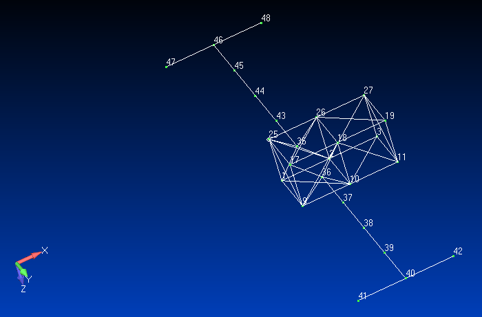
For this example, we’ll use a simple space-station model that has been reduced into two separate Hurty-Craig-Bampton models: an “inboard” model and an “outboard” model. These model attach at nodes 3, 11, 19, and 27.
Notes:
These model use units of kg, mm, s
They are very light-weight trusses:
Mass of inboard model = 1.755 kg
Mass of outboard model = 1.590 kg
The inboard model (the Source):

The outboard model (the Load):
First, do some imports:
import inspect
from pathlib import Path
from io import StringIO
import numpy as np
from scipy import linalg as la
import matplotlib.pyplot as plt
import pandas as pd
from pyyeti import cb, frclim, ode, ytools
from pyyeti.nastran import bulk, op4, n2p
from pyyeti.pp import PP
Some settings specifically for the jupyter notebook:
%matplotlib inline
plt.rcParams['figure.figsize'] = [6.4, 4.8]
plt.rcParams['figure.dpi'] = 150.
Need path to data files:
srcdir = Path(inspect.getfile(frclim)).parent / "tests" / "nas2cam_extseout"
Load model data
Also add 2% critical modal damping for both models:
zeta = 0.02
ids = ("out", "in")
uset, cords, b = {}, {}, {}
mats = {}
for id in ids:
    uset[id], cords[id], b[id] = bulk.asm2uset(srcdir / f"{id}board.asm")
    mats[id] = op4.read(srcdir / f"{id}board.op4")

    # add damping:
    bxx = 0 * mats[id]["kxx"]
    q = ~b[id]
    lam = np.diag(mats[id]["kxx"])[q]
    damp = 2 * np.sqrt(lam) * zeta
    bxx[q, q] = damp
    mats[id]["bxx"] = bxx

PP(mats, 2);
<class 'dict'>[n=2]
    'out': <class 'collections.OrderedDict'>[n=30]
        'kxx'   : float64 ndarray 2116 elems: (46, 46)
        'mxx'   : float64 ndarray 2116 elems: (46, 46)
        'bxx1'  : float64 ndarray 1 elems: (1, 1) [[ 0.]]
        'k4xx1' : float64 ndarray 1 elems: (1, 1) [[ 0.]]
        'px1'   : float64 ndarray 1 elems: (1, 1) [[ 0.]]
        'gpxx'  : float64 ndarray 1 elems: (1, 1) [[ 0.]]
        'gdxx'  : float64 ndarray 1 elems: (1, 1) [[ 0.]]
        'rvax'  : float64 ndarray 1 elems: (1, 1) [[ 0.]]
        'va'    : float64 ndarray 46 elems: (46, 1)
        'mug1'  : float64 ndarray 1932 elems: (42, 46)
        'mug1o' : float64 ndarray 1 elems: (1, 1) [[ 0.]]
        'mes1'  : float64 ndarray 1 elems: (1, 1) [[ 0.]]
        'mes1o' : float64 ndarray 1 elems: (1, 1) [[ 0.]]
        'mee1'  : float64 ndarray 1 elems: (1, 1) [[ 0.]]
        'mee1o' : float64 ndarray 1 elems: (1, 1) [[ 0.]]
        'mgpfm' : float64 ndarray 1 elems: (1, 1) [[ 0.]]
        'mgpfb' : float64 ndarray 1 elems: (1, 1) [[ 0.]]
        'mgpfk' : float64 ndarray 1 elems: (1, 1) [[ 0.]]
        'mgpfo' : float64 ndarray 1 elems: (1, 1) [[ 0.]]
        'mef1'  : float64 ndarray 1104 elems: (24, 46)
        'mef1o' : float64 ndarray 1 elems: (1, 1) [[ 0.]]
        'mqgm'  : float64 ndarray 1 elems: (1, 1) [[ 0.]]
        'mqgb'  : float64 ndarray 1 elems: (1, 1) [[ 0.]]
        'mqgk'  : float64 ndarray 1 elems: (1, 1) [[ 0.]]
        'mqg1o' : float64 ndarray 1 elems: (1, 1) [[ 0.]]
        'mqmgm' : float64 ndarray 1 elems: (1, 1) [[ 0.]]
        'mqmgb' : float64 ndarray 1 elems: (1, 1) [[ 0.]]
        'mqmgk' : float64 ndarray 1 elems: (1, 1) [[ 0.]]
        'mqmg1o': float64 ndarray 1 elems: (1, 1) [[ 0.]]
        'bxx'   : float64 ndarray 2116 elems: (46, 46)
    'in' : <class 'collections.OrderedDict'>[n=30]
        'kxx'   : float64 ndarray 1024 elems: (32, 32)
        'mxx'   : float64 ndarray 1024 elems: (32, 32)
        'bxx1'  : float64 ndarray 1 elems: (1, 1) [[ 0.]]
        'k4xx1' : float64 ndarray 1 elems: (1, 1) [[ 0.]]
        'px'    : float64 ndarray 960 elems: (32, 30)
        'gpxx'  : float64 ndarray 1 elems: (1, 1) [[ 0.]]
        'gdxx'  : float64 ndarray 1 elems: (1, 1) [[ 0.]]
        'rvax'  : float64 ndarray 1 elems: (1, 1) [[ 0.]]
        'va'    : float64 ndarray 32 elems: (32, 1)
        'mug1'  : float64 ndarray 1152 elems: (36, 32)
        'mug1o' : float64 ndarray 1 elems: (1, 1) [[ 0.]]
        'mes1'  : float64 ndarray 864 elems: (27, 32)
        'mes1o' : float64 ndarray 1 elems: (1, 1) [[ 0.]]
        'mee1'  : float64 ndarray 1 elems: (1, 1) [[ 0.]]
        'mee1o' : float64 ndarray 1 elems: (1, 1) [[ 0.]]
        'mgpfm' : float64 ndarray 1 elems: (1, 1) [[ 0.]]
        'mgpfb' : float64 ndarray 1 elems: (1, 1) [[ 0.]]
        'mgpfk' : float64 ndarray 1 elems: (1, 1) [[ 0.]]
        'mgpfo' : float64 ndarray 1 elems: (1, 1) [[ 0.]]
        'mef1'  : float64 ndarray 512 elems: (16, 32)
        'mef1o' : float64 ndarray 1 elems: (1, 1) [[ 0.]]
        'mqgm'  : float64 ndarray 1 elems: (1, 1) [[ 0.]]
        'mqgb'  : float64 ndarray 1 elems: (1, 1) [[ 0.]]
        'mqgk'  : float64 ndarray 1 elems: (1, 1) [[ 0.]]
        'mqg1o' : float64 ndarray 1 elems: (1, 1) [[ 0.]]
        'mqmgm' : float64 ndarray 1 elems: (1, 1) [[ 0.]]
        'mqmgb' : float64 ndarray 1 elems: (1, 1) [[ 0.]]
        'mqmgk' : float64 ndarray 1 elems: (1, 1) [[ 0.]]
        'mqmg1o': float64 ndarray 1 elems: (1, 1) [[ 0.]]
        'bxx'   : float64 ndarray 1024 elems: (32, 32)
For convenience and ease of reading, create some shorter names for the mass, damping, and stiffness matrices:
maa = {
    "in": mats["in"]["mxx"],
    "out": mats["out"]["mxx"],
}
kaa = {
    "in": mats["in"]["kxx"],
    "out": mats["out"]["kxx"],
}
baa = {
    "in": mats["in"]["bxx"],
    "out": mats["out"]["bxx"],
}
Model checks
We’ll use the pyyeti.cb.cbcheck routine to run model checks on both models. (There is also a tutorial on running model checks here). For this notebook, the primary reason for running model checks was simply to get the modal effective mass tables since that data may be helpful in interpreting some of the plots below. However, pyyeti.cb.cbcheck also turned out to be helpful in diagnosing an numerical issue with the inboard model; more on that in a moment. First, run the model checks and display the modal effective mass tables:
bset_in = b["in"].nonzero()[0]
bset_out = b["out"].nonzero()[0]

with StringIO() as f:
    chk_in = cb.cbcheck(
        f,  # "cbcheck_in.txt",
        maa["in"],
        kaa["in"],
        bset_in,
        bset_in[:6],
        uset["in"],
        uref=[600, 150, 150],  # this is the center if the 4 i/f nodes
        rb_norm=True,
    )
    str_chk_in = f.getvalue()

with StringIO() as f:
    chk_out = cb.cbcheck(
        f,  # "cbcheck_out.txt",
        maa["out"],
        kaa["out"],
        bset_out,
        bset_out[:6],
        uset["out"],
        uref=[600, 150, 150],
        rb_norm=True,
    )
    str_chk_out = f.getvalue()
Iteration 1 completed
Convergence: 4 of 6, tolerance range after 2 iterations is [1.196996633817e-09, 1.190690665692671e-05]
Convergence: 6 of 6, tolerance range after 3 iterations is [3.4365399102737635e-12, 2.7573499099751664e-11]
Show the modal effective mass tables:
pd.options.display.float_format = '{:,.2f}'.format
chk_in.effmass_percent
| T1 | T2 | T3 | R1 | R2 | R3 | |
|---|---|---|---|---|---|---|
| Frq (Hz) | ||||||
| 6.13 | 0.00 | 31.93 | 6.06 | 0.00 | 15.61 | 82.15 |
| 6.13 | 0.00 | 6.06 | 31.93 | 0.00 | 82.14 | 15.60 |
| 23.63 | 0.00 | 0.00 | 0.00 | 80.42 | 0.00 | 0.00 |
| 70.48 | 0.00 | 31.05 | 0.56 | 0.00 | 0.03 | 1.67 |
| 70.79 | 0.00 | 0.56 | 31.25 | 0.00 | 1.68 | 0.03 |
| 104.67 | 44.16 | 0.00 | 0.00 | 0.00 | 0.00 | 0.00 |
| 188.04 | 0.63 | 0.08 | 0.00 | 0.00 | 0.00 | 0.01 |
| 208.60 | 0.00 | 0.38 | 0.00 | 0.00 | 0.00 | 0.01 |
chk_out.effmass_percent
| T1 | T2 | T3 | R1 | R2 | R3 | |
|---|---|---|---|---|---|---|
| Frq (Hz) | ||||||
| 1.65 | 0.00 | 0.00 | 0.00 | 0.00 | 0.00 | 46.18 |
| 1.65 | 11.86 | 0.00 | 0.00 | 0.00 | 0.00 | 0.00 |
| 1.67 | 0.00 | 0.00 | 0.00 | 83.95 | 0.00 | 0.00 |
| 1.67 | 0.00 | 0.00 | 12.24 | 0.00 | 12.34 | 0.00 |
| 7.03 | 0.00 | 0.00 | 0.00 | 0.00 | 0.88 | 0.00 |
| 7.03 | 0.00 | 0.00 | 0.00 | 0.00 | 0.00 | 0.00 |
| 10.91 | 0.00 | 0.00 | 0.00 | 0.00 | 0.00 | 1.52 |
| 10.91 | 2.47 | 0.00 | 0.00 | 0.00 | 0.00 | 0.00 |
| 13.99 | 0.00 | 0.00 | 0.00 | 2.69 | 0.00 | 0.00 |
| 13.99 | 0.00 | 0.00 | 2.76 | 0.00 | 2.78 | 0.00 |
| 25.13 | 0.00 | 0.00 | 0.00 | 0.00 | 0.00 | 0.42 |
| 25.14 | 0.99 | 0.00 | 0.00 | 0.00 | 0.00 | 0.00 |
| 42.17 | 0.00 | 0.00 | 0.00 | 0.51 | 0.00 | 0.00 |
| 42.19 | 0.00 | 0.00 | 1.01 | 0.00 | 1.02 | 0.00 |
| 46.72 | 0.00 | 5.38 | 0.00 | 0.00 | 0.00 | 2.75 |
| 46.89 | 0.00 | 0.00 | 0.00 | 0.00 | 0.00 | 0.00 |
| 69.17 | 0.00 | 0.12 | 0.00 | 0.00 | 0.00 | 0.98 |
| 87.50 | 5.08 | 0.00 | 0.00 | 0.00 | 0.00 | 0.00 |
| 110.85 | 0.00 | 81.36 | 0.44 | 0.00 | 0.32 | 45.80 |
| 139.24 | 0.00 | 0.69 | 70.30 | 0.00 | 76.14 | 0.16 |
| 152.23 | 1.14 | 0.00 | 0.00 | 8.66 | 0.00 | 0.00 |
| 472.62 | 0.00 | 0.01 | 0.67 | 0.00 | 2.50 | 0.03 |
A quick look at the first few lines of the output:
print(str_chk_in[:str_chk_in.index("\n\n")])
Mass matrix is symmetric.
Warning: mass matrix is not positive-definite.
    However, subspace iteration succeeded, which means the mass
    must be close to positive-definite.
Warning: stiffness matrix is not symmetric: abs-max-err = 5.96e-07
print(str_chk_out[:str_chk_out.index("\n\n")])
Mass matrix is symmetric.
Mass matrix is positive-definite.
Stiffness matrix is symmetric.
The model checks showed that the inboard model mass and stiffness were not perfect: the mass was not positive-definite (but close), and the stiffness was not symmetric (but close). However, since they were close, all the model checks ran fine and show that the model is good. Why did the matrices come out this way? That’s how Nastran wrote them and they are fine as far as Nastran is concerned. These Python routines however look for a higher degree of precision. (It’s possible that converting units from millimeters to meters may avoid this issue by providing better relative scaling but, at the time of this writing, that has not been tried.)
Because of the numerical imperfections, we’ll get a warning below from the pyyeti.frclim.calcAM routine about having trouble using the pyyeti.ode.SolveUnc solver to compute the apparent mass. After issuing the warning, it will automatically switch to the pyyeti.ode.FreqDirect solver to successfully compute the apparent mass. The reason that pyyeti.cb.cbcheck succeeded in solving the eigenproblem while pyyeti.ode.SolveUnc did not is simply because they use different eigen solvers: pyyeti.cb.cbcheck uses pyyeti.ytools.eig_si, which has some leniency built-in, while pyyeti.ode.SolveUnc uses scipy.linalg.eigh, which is very strict.
Since it’s illuminating, we’ll show how close the mass matrix is to positive-definite by making a tiny modification to it, similar to what pyyeti.ytools.eig_si does. We’ll increase the diagonal values by a tiny amount:
m = maa['in'].copy()
print(f"Before: {ytools.mattype(m, 'posdef') = }")
d = np.arange(m.shape[0])
m[d, d] *= 1.000000000000001
print(f"After: {ytools.mattype(m, 'posdef') = }")
Before: ytools.mattype(m, 'posdef') = False
After: ytools.mattype(m, 'posdef') = True
Define the forcing function
We’ll use the first TLOAD vector of “inboard” to apply a force to the coupled system. This load vector applies forces to nodes 13 & 21. For simplicity, we’ll keep the forces constant across the frequency range.
The analysis will cover the frequency range 0.01 to 100.0 Hz on a logarithmic scale.
freq = np.geomspace(0.01, 100.0, 4 * 167 + 1)

# use first TLOAD vector and expand it:
force_in = mats["in"]["px"][:, :1] @ np.ones((1, len(freq)))
force_in.shape
(32, 669)
Take a quick look at the inboard applied forces:
np.set_printoptions(precision=3, linewidth=130, suppress=True)
force_in[:, :5]
array([[  11.615,   11.615,   11.615,   11.615,   11.615],
       [   0.158,    0.158,    0.158,    0.158,    0.158],
       [  -6.209,   -6.209,   -6.209,   -6.209,   -6.209],
       [-334.015, -334.015, -334.015, -334.015, -334.015],
       [-680.302, -680.302, -680.302, -680.302, -680.302],
       [-417.33 , -417.33 , -417.33 , -417.33 , -417.33 ],
       [  -0.204,   -0.204,   -0.204,   -0.204,   -0.204],
       [   6.209,    6.209,    6.209,    6.209,    6.209],
       [  -9.713,   -9.713,   -9.713,   -9.713,   -9.713],
       [ 619.975,  619.975,  619.975,  619.975,  619.975],
       [-291.083, -291.083, -291.083, -291.083, -291.083],
       [-359.031, -359.031, -359.031, -359.031, -359.031],
       [ -11.615,  -11.615,  -11.615,  -11.615,  -11.615],
       [   4.454,    4.454,    4.454,    4.454,    4.454],
       [  -1.912,   -1.912,   -1.912,   -1.912,   -1.912],
       [ -92.337,  -92.337,  -92.337,  -92.337,  -92.337],
       [-739.591, -739.591, -739.591, -739.591, -739.591],
       [-358.041, -358.041, -358.041, -358.041, -358.041],
       [   9.713,    9.713,    9.713,    9.713,    9.713],
       [   4.092,    4.092,    4.092,    4.092,    4.092],
       [   1.912,    1.912,    1.912,    1.912,    1.912],
       [ -67.321,  -67.321,  -67.321,  -67.321,  -67.321],
       [ 679.264,  679.264,  679.264,  679.264,  679.264],
       [-231.794, -231.794, -231.794, -231.794, -231.794],
       [  -5.2  ,   -5.2  ,   -5.2  ,   -5.2  ,   -5.2  ],
       [   1.575,    1.575,    1.575,    1.575,    1.575],
       [ -10.157,  -10.157,  -10.157,  -10.157,  -10.157],
       [   5.768,    5.768,    5.768,    5.768,    5.768],
       [  -0.037,   -0.037,   -0.037,   -0.037,   -0.037],
       [   0.603,    0.603,    0.603,    0.603,    0.603],
       [  -7.554,   -7.554,   -7.554,   -7.554,   -7.554],
       [  -5.275,   -5.275,   -5.275,   -5.275,   -5.275]])
Couple models together the old fashioned way:
We’ll define a matrix ‘S’ that will enforce boundary compatibility. It defines the relationship from the DOF chosen to be the independent set (\(p_{ind}\)) to all the DOF (\(p_{all}\)):
Since \(out_b = in_b\):
The following code takes advantage of the fact that the b-set is ordered first for both models.
m = maa["in"].shape[0]
n = maa["out"].shape[0]
nb = np.count_nonzero(b["in"])
S = {}
S["in"] = np.block(
    [
        [np.eye(nb), np.zeros((nb, m + n - 2 * nb))],
        [np.zeros((m - nb, nb)), np.eye(m - nb), np.zeros((m - nb, n - nb))],
    ]
)
S["out"] = np.block(
    [
        [np.eye(nb), np.zeros((nb, m + n - 2 * nb))],
        [np.zeros((n - nb, m)), np.eye(n - nb)],
    ]
)
S["tot"] = np.vstack((S["in"], S["out"]))
Apply the S matrix to couple the models together:
mc = S["tot"].T @ la.block_diag(maa["in"], maa["out"]) @ S["tot"]
kc = S["tot"].T @ la.block_diag(kaa["in"], kaa["out"]) @ S["tot"]
bc = S["tot"].T @ la.block_diag(baa["in"], baa["out"]) @ S["tot"]
As a check, compare coupled model frequencies to Nastran:
lam, phi = la.eigh(kc, mc)
freqsys = np.sqrt(abs(lam)) / 2 / np.pi
eigen = bulk.rdeigen(srcdir / "assemble.out")
np.allclose(freqsys[6:], eigen[0]["cycles"][6:])
True
The system frequencies up to 110 Hz:
pv = eigen[0]["cycles"] <= 110.0
eigen[0][["cycles"]][pv]
| cycles | |
|---|---|
| 1 | 0.00 |
| 2 | 0.00 |
| 3 | 0.00 |
| 4 | 0.00 |
| 5 | 0.00 |
| 6 | 0.00 |
| 7 | 1.70 |
| 8 | 1.77 |
| 9 | 1.86 |
| 10 | 3.42 |
| 11 | 7.02 |
| 12 | 7.03 |
| 13 | 10.72 |
| 14 | 10.98 |
| 15 | 13.87 |
| 16 | 14.39 |
| 17 | 14.65 |
| 18 | 15.19 |
| 19 | 25.20 |
| 20 | 25.31 |
| 21 | 29.13 |
| 22 | 42.44 |
| 23 | 43.09 |
| 24 | 46.89 |
| 25 | 47.81 |
| 26 | 69.45 |
| 27 | 87.46 |
| 28 | 97.91 |
| 29 | 100.85 |
Solve the equations of motion the old fashioned way
We’ll solve the equations of motion using pyyeti.ode.SolveUnc and recover responses for both components. Note that upstream data recovery could be done easily with the “mug1”, “mef1” and “mes1” matrices loaded from the op4 files above.
fs = ode.SolveUnc(mc, bc, kc, pre_eig=True)
force = S["in"].T @ force_in
sol = fs.fsolve(force, freq, incrb="avd")  # keep all rb responses for demo

# recover displacements, velocities, and accelerations for both components:
d, v, a = {}, {}, {}
ifforce = {}
for id in ids:
    d[id] = S[id] @ sol.d
    v[id] = S[id] @ sol.v
    a[id] = S[id] @ sol.a

    ifforce[id] = (maa[id] @ a[id] + baa[id] @ v[id] + kaa[id] @ d[id])[:nb]
Do some sanity checks on the results. The boundary accelerations, velocities, and displacements should match, and the boundary forces from one component on the other should be equal and opposite.
print(f'{np.allclose(a["in"][:nb], a["out"][:nb]) = }')
print(f'{np.allclose(v["in"][:nb], v["out"][:nb]) = }')
print(f'{np.allclose(d["in"][:nb], d["out"][:nb]) = }')

print()
print(f'{np.allclose(-ifforce["out"], ifforce["in"] - force[:nb]) = }')
print(f'{abs(ifforce["out"] + (ifforce["in"] - force[:nb])).max() = }')

pv = freq >= 1.0
print()
print(f'For freq >= 1.0:\n\t{np.allclose(-ifforce["out"][:, pv], ifforce["in"][:, pv] - force[:nb, pv]) = }')
np.allclose(a["in"][:nb], a["out"][:nb]) = True
np.allclose(v["in"][:nb], v["out"][:nb]) = True
np.allclose(d["in"][:nb], d["out"][:nb]) = True

np.allclose(-ifforce["out"], ifforce["in"] - force[:nb]) = False
abs(ifforce["out"] + (ifforce["in"] - force[:nb])).max() = 0.0029273294523193272

For freq >= 1.0:
    np.allclose(-ifforce["out"][:, pv], ifforce["in"][:, pv] - force[:nb, pv]) = True
Note:
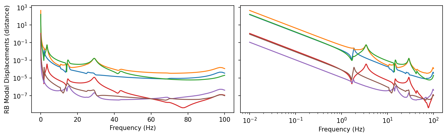
In the lowest frequencies, we lose some numerical precision on the boundary forces if we set
incrb = "avd"in the call to fsolve above (the default). That’s because the rigid-body displacements will grow to infinity as frequency approaches zero. This is shown in the next plot; both linear and log scales are shown for the x-axis scales because it is interesting and informative. We’ll explore a similar phenomenon a little more later in the NT context. For now, we’ll note that the forces are still very close and that above 1.0 Hz, even withincrb = "avd", thenp.allclosecheck passes.
fig = plt.figure("RB Modal Displacements", clear=True, layout="constrained", figsize=(10, 3))
axes = fig.subplots(1, 2, sharey=True)
axes[0].semilogy(freq, abs(d['out'][:6].T))
axes[1].loglog(freq, abs(d['out'][:6].T))
axes[0].set_xlabel("Frequency (Hz)")
axes[1].set_xlabel("Frequency (Hz)")
axes[0].set_ylabel("RB Modal Displacements (distance)");
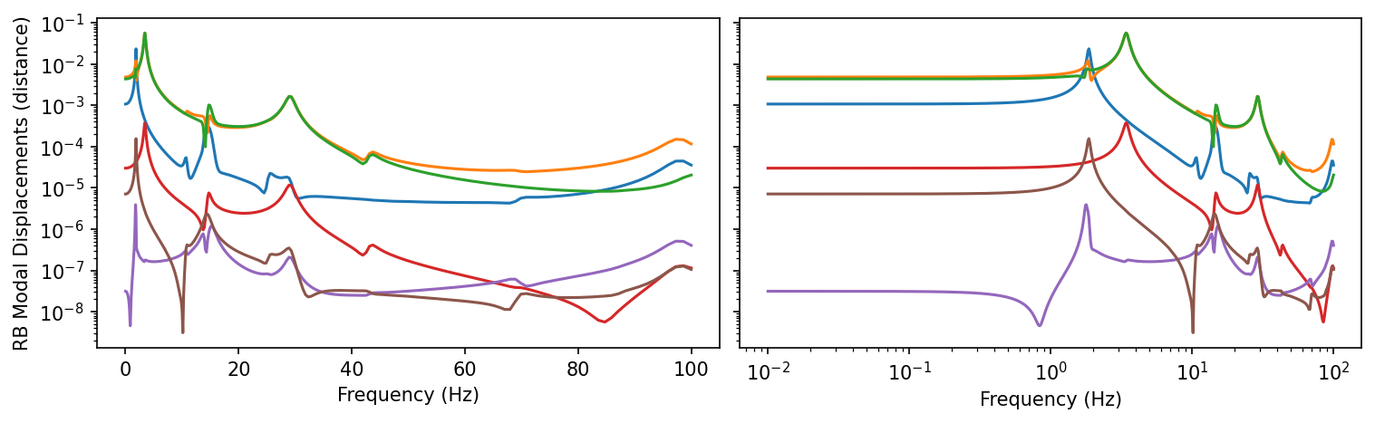
Repeat the above, but with incrb = "av" in the call to
fsolve:
fs = ode.SolveUnc(mc, bc, kc, pre_eig=True)
force = S["in"].T @ force_in
sol = fs.fsolve(force, freq, incrb="av")  # zero out the rb displacements

# recover displacements, velocities, and accelerations for both components:
d, v, a = {}, {}, {}
ifforce = {}
for id in ids:
    d[id] = S[id] @ sol.d
    v[id] = S[id] @ sol.v
    a[id] = S[id] @ sol.a

    ifforce[id] = (maa[id] @ a[id] + baa[id] @ v[id] + kaa[id] @ d[id])[:nb]

print(f'{np.allclose(-ifforce["out"], ifforce["in"] - force[:nb]) = }')
print(f'{abs(ifforce["out"] + (ifforce["in"] - force[:nb])).max() = }')

fig = plt.figure("RB Modal Displacements", clear=True, layout="constrained", figsize=(10, 3))
axes = fig.subplots(1, 2, sharey=True)
axes[0].semilogy(freq, abs(d['out'][:6].T))
axes[1].loglog(freq, abs(d['out'][:6].T))
axes[0].set_xlabel("Frequency (Hz)")
axes[1].set_xlabel("Frequency (Hz)")
axes[0].set_ylabel("RB Modal Displacements (distance)");
np.allclose(-ifforce["out"], ifforce["in"] - force[:nb]) = True
abs(ifforce["out"] + (ifforce["in"] - force[:nb])).max() = 1.7281315377588588e-07
Use the NT approach to couple models together
First, we’ll compute the “free acceleration” \(A_s\):
fs_in = ode.FreqDirect(maa["in"], baa["in"], kaa["in"])
As = fs_in.fsolve(force_in, freq).a[:nb]
Next, we’ll compute the apparent masses and call pyyeti.frclim.ntfl to compute coupled system responses.
For illustration and as a check on the routine, we’ll use both methods
within
pyyeti.frclim.calcAM
to compute the apparent masses. Those two methods are labeled as
cbtf and fsolve here; for more information, see
pyyeti.frclim.calcAM.
Note that we’ll get a warning from pyyeti.frclim.calcAM about switching to the pyyeti.ode.FreqDirect solver. See above for more discussion on this.
AM = {}
NT = {}
for method in ("cbtf", "fsolve"):
    AM[method] = {}
    for id in ids:
        if method == "cbtf":
            drm = np.arange(nb)
        else:
            drm = np.zeros((nb, maa[id].shape[0]))
            drm[:, b[id]] = np.eye(nb)
        AM[method][id] = frclim.calcAM([maa[id], baa[id], kaa[id], drm], freq)

    NT[method] = frclim.ntfl(AM[method]["in"], AM[method]["out"], As, freq)
/home/docs/checkouts/readthedocs.org/user_builds/pyyeti/envs/latest/lib/python3.12/site-packages/pyyeti/frclim.py:231: RuntimeWarning: Switching from `SolveUnc` to `FreqDirect` because complex eigensolver failed; see messages above. Solution may be slow.
  warnings.warn(
Perform some sanity checks and comparisons against the “CLA” (old
fashioned) approach. Again, we see some loss of numerical precision at
the lowest frequencies as we noted above for the CLA approach when we
used incrb="dav". We’ll discuss this below.
for method in NT:
    print()
    print(method)
    print(f'\t{np.allclose(ifforce["out"][:, pv], NT[method].F[:, pv]) = }')
    print(f'\t{np.allclose(a["out"][:nb, pv], NT[method].A[:, pv]) = }')
    print(f'\t{abs(ifforce["out"] - NT[method].F).max() = }')
    print(f'\t{abs(a["out"][:nb] - NT[method].A).max() = }')
cbtf
    np.allclose(ifforce["out"][:, pv], NT[method].F[:, pv]) = True
    np.allclose(a["out"][:nb, pv], NT[method].A[:, pv]) = True
    abs(ifforce["out"] - NT[method].F).max() = 4.8351414481562216e-05
    abs(a["out"][:nb] - NT[method].A).max() = 2.4382675478551441e-05

fsolve
    np.allclose(ifforce["out"][:, pv], NT[method].F[:, pv]) = True
    np.allclose(a["out"][:nb, pv], NT[method].A[:, pv]) = True
    abs(ifforce["out"] - NT[method].F).max() = 0.00013002828172092862
    abs(a["out"][:nb] - NT[method].A).max() = 2.1016948736907182e-05
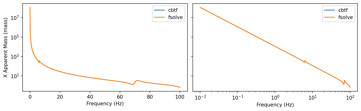
As noted above, we lose some numerical precision in the lowest
frequencies. In the NT approach, this appears to be due to very large
apparent mass values. To illustrate, here are the apparent mass curves
for both approaches for the x DOF of the first boundary node for the
Source model.
It’s plotted on two different scales because it’s interesting and informative.
fig = plt.figure("AM", clear=True, layout="constrained", figsize=(10, 3))
axes = fig.subplots(1, 2, sharey=True)
for method in AM:
    axes[0].semilogy(freq, abs(AM[method]["in"][0, :, 0]), label=method)
    axes[1].loglog(freq, abs(AM[method]["in"][0, :, 0]), label=method)
axes[0].legend()
axes[1].legend()
axes[0].set_xlabel("Frequency (Hz)")
axes[1].set_xlabel("Frequency (Hz)")
axes[0].set_ylabel("X Apparent Mass (mass)");
Similarly, for the Load model:
fig = plt.figure("AM", clear=True, layout="constrained", figsize=(10, 3))
axes = fig.subplots(1, 2, sharey=True)
for method in AM:
    axes[0].semilogy(freq, abs(AM[method]["out"][0, :, 0]), label=method)
    axes[1].loglog(freq, abs(AM[method]["out"][0, :, 0]), label=method)
axes[0].legend()
axes[1].legend()
axes[0].set_xlabel("Frequency (Hz)")
axes[1].set_xlabel("Frequency (Hz)")
axes[0].set_ylabel("X Apparent Mass (mass)");

One way to think about the apparent mass is that it is the set of forces required to enforce a unit acceleration on one boundary DOF while restraining all other boundary DOF. (That would be one column of the apparent mass matrix at a particular frequency.) In other words, in \(f = m a\), if \(a = \mathbf{I}\), then the apparent mass \(m\) is equal to the force \(f\). As frequency approaches zero, the structure will respond statically to the slowly oscillating sinusoidal forces and the relation between the displacement and the force is:
Since \(a = -\omega^2 x\):
So, as frequency approaches zero, the apparent mass will increase proportionally to \(1/\omega^2\), which explains the straight line slope on the log-log plot (see also the next plot).
Note that for statically-determinate interfaces, the apparent mass simply approaches the rigid-body mass as frequency approaches 0.0 Hz since the system will move as a rigid-body.
However, even down to 0.01 Hz, the results for the NT approaches are
still quite close, and above 1.0 Hz, all the np.allclose checks
return True.
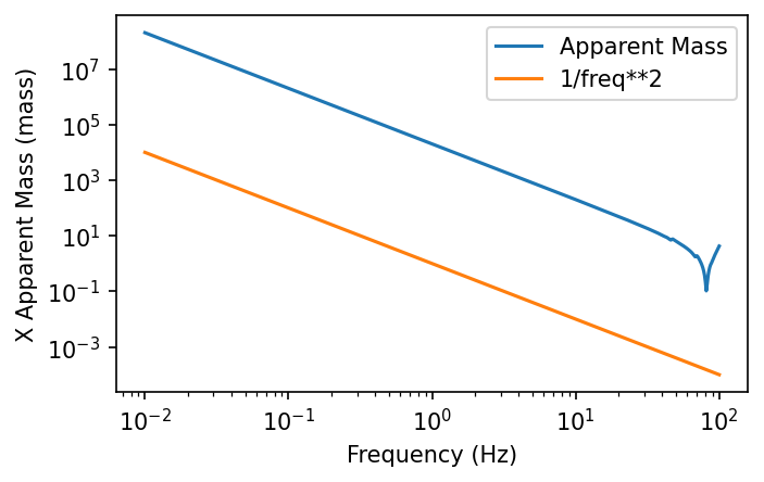
For illustration, here is a plot showing the slope of the apparent mass is indeed proportional to \(1/\omega^2\):
fig = plt.figure(figsize=(5, 3))
axes = fig.subplots(1, 1)
axes.semilogy(freq, abs(AM["cbtf"]["out"][0, :, 0]), label="Apparent Mass")
axes.loglog(freq, 1/freq**2, label="1/freq**2")
axes.legend()
axes.set_xlabel("Frequency (Hz)")
axes.set_ylabel("X Apparent Mass (mass)");
Plot interface forces and accelerations
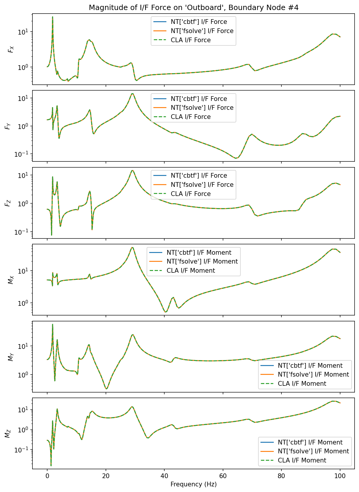
For illustration, we’ll plot some of the interface forces and boundary accelerations. We can see that NT responses are the same as the CLA responses.
First, compare the interface forces for the 4th boundary node (as an example):
fig = plt.figure("ifforce", clear=True, layout="constrained", figsize=(8, 11))
frcaxes = fig.subplots(6, 1, sharex=True)

ylabels = ["$F_X$", "$F_Y$", "$F_Z$", "$M_X$", "$M_Y$", "$M_Z$"]
node = 4
for j, ax in enumerate(frcaxes):
    row = j + (node - 1) * 6
    which = "Force" if ylabels[j].startswith("$F") else "Moment"
    for method in NT:
        ax.semilogy(
            freq, abs(NT[method].F[row]), label=f"NT[{method!r}] I/F {which}"
        )
    ax.semilogy(freq, abs(ifforce["out"][row]), "--", label=f"CLA I/F {which}")
    ax.legend()
    ax.set_ylabel(ylabels[j])

frcaxes[0].set_title(f"Magnitude of I/F Force on 'Outboard', Boundary Node #{node}")
frcaxes[-1].set_xlabel("Frequency (Hz)");
Next, compare the interface accelerations for the 4th boundary node. For reference, the free acceleration for this node is also plotted:
fig = plt.figure("ifacce", clear=True, layout="constrained", figsize=(8, 11))
acceaxes = fig.subplots(6, 1, sharex=True)

ylabels = ["$A_{X}$", "$A_{Y}$", "$A_{Z}$", "$A_{RX}$", "$A_{RY}$", "$A_{RZ}$"]
for j, ax in enumerate(acceaxes):
    row = j + (node - 1) * 6
    for method in NT:
        ax.semilogy(
            freq, abs(NT[method].A[row]), label=f"NT[{method!r}] Coupled Acce"
        )
    ax.semilogy(freq, abs(a["out"][row]), "--", label="CLA Coupled Acce")
    ax.semilogy(freq, abs(As[row]), label="Free Acce")
    ax.legend()
    ax.set_ylabel(ylabels[j])

acceaxes[0].set_title(f"Magnitude of I/F Acceleration, Boundary Node #{node}")
acceaxes[-1].set_xlabel("Frequency (Hz)");
