pyyeti.dsp.fftcoef

pyyeti.dsp.fftcoef(x, sr, *, axis=-1, coef='mag', window='boxcar', dodetrend=False, fold=True, maxdf=None)

FFT sine/cosine or magnitude/phase coefficients of a real signal

This routine returns the positive frequency coefficients only.

Parameters:

• x (nd array_like) – The (real) signal(s) to FFT. The FFT is carried out along axis axis.

• sr (scalar) – The sample rate (samples/sec)

• axis (int, optional) – Axis along which to operate.

• coef (string; optional) – Specifies how to return the coefficients:

  coef	Return
  “mag”	(magnitude, phase, freq)
  “ab”	(a, b, freq)
  “complex”	(a + i b, None, freq)

  See below for more details.

• window (string, tuple, or 1d array_like; optional) – Specifies window function. If a string or tuple, it is passed to scipy.signal.get_window() to get the window. If 1d array_like, it must be length len(x) and is used directly.

• dodetrend (bool; optional) – If True, remove a linear fit from x; otherwise, no detrending is done.

• fold (bool; optional) – If true, “fold” negative frequencies on top of positive frequencies such that the coefficients at frequencies that have a negative counterpart are doubled (magnitude is also doubled).

• maxdf (scalar or None; optional) – If scalar, this is the maximum allowed frequency step; zero padding will be done if necessary to enforce this. Note that this is for providing more points between peaks only. If None, the delta frequency is simply sr/len(x).

Returns:

3-tuple depending on coef –

coef	Return value
”mag”	(magnitude, phase, freq)
”ab”	(a, b, freq)
”complex”	(a + i b, None, freq)

All values are for the positive side frequencies only. The dimensions of the nd arrays magnitude, phase, a and b are similar to input x except that along the axis axis; the dimension of that axis corresponds to freq. freq is a 1d array of the positive side frequencies only.

Definitions of magnitude, phase, and the a and b coefficients are shown below. freq is in Hz.

Notes

The FFT results are scaled according to the ‘coherent gain’ of the window function. For the “boxcar” window (which is just all 1.0’s), the coherent gain is 1.0. The coherent gain is defined by:

scale = 1/coherent_gain
coherent_gain = sum(window)/len(window)

The coefficients are related to the original signal by either of these two equivalent summations (if fold is True):

\[x(t_n) = \sum\limits^{len(x)-1}_{k=0} A_k \cos(k \omega t_n) + B_k \sin(k \omega t_n)\]

\[x(t_n) = \sum\limits^{len(x)-1}_{k=0} M_k\sin(k \omega t_n - \phi_k)\]

where \(\omega = 2 \pi \Delta freq\), \(M\) is the magnitude, and \(\phi\) is the phase. The magnitude and phase are computed by:

\[ \begin{align}\begin{aligned}\begin{aligned} M_k &= \sqrt {A_k^2 + B_k^2}\\\phi_k &= \arctan2(-A_k, B_k) \end{aligned}\end{aligned}\end{align} \]

Normally, the frequency step is defined by:

\[\Delta freq = sr / \text{len}(x)\]

A finer frequency step can be achieved by specifying the maxdf parameter. If maxdf is specified and the frequency step computed from the above equation is greater than maxdf, the frequency step is computed by:

\[ \begin{align}\begin{aligned}\begin{aligned} N &= \text{nextpow2}(\text{int}(sr / maxdf))\\\Delta freq &= sr / N \end{aligned}\end{aligned}\end{align} \]

The function nextpow2() finds the next power of 2 integer. This approach makes efficient use of the FFT while ensuring the final frequency step is less than or equal to maxdf.

The example below uses these formulas directly to upsample a signal. This is for demonstration only; to truly upsample a signal based on FFT in a more efficient manner, see scipy.signal.resample(). (See also resample().)

See also

fftmap(), transmissibility()

Examples

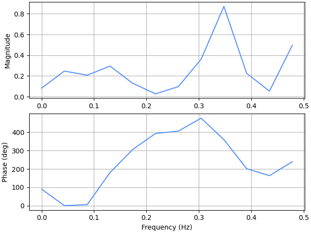
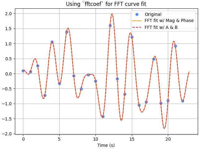
>>> import numpy as np
>>> import matplotlib.pyplot as plt
>>> from pyyeti import dsp
>>> n = 23
>>> rng = np.random.default_rng()
>>> x = rng.normal(size=n)
>>> t = np.arange(n)
>>> mag, phase, frq = dsp.fftcoef(x, 1.0)
>>> _ = plt.figure('Example', clear=True, layout='constrained')
>>> _ = plt.subplot(211)
>>> _ = plt.plot(frq, mag)
>>> _ = plt.ylabel('Magnitude')
>>> _ = plt.subplot(212)
>>> _ = plt.plot(frq, np.rad2deg(np.unwrap(phase)))
>>> _ = plt.ylabel('Phase (deg)')
>>> _ = plt.xlabel('Frequency (Hz)')
>>>
>>> w = 2*np.pi*frq[1]
>>>
>>> # use a finer time vector for reconstructions:
>>> t2 = np.arange(0., n, .05)
>>>
>>> # reconstruct with magnitude and phase:
>>> x2 = 0.0
>>> for k, (m, p, f) in enumerate(zip(mag, phase, frq)):
...     x2 = x2 + m*np.sin(k*w*t2 - p)
>>>
>>> # reconstruct with A and B:
>>> A, B, frq = dsp.fftcoef(x, 1.0, coef='ab')
>>> x3 = 0.0
>>> for k, (a, b, f) in enumerate(zip(A, B, frq)):
...     x3 = x3 + a*np.cos(k*w*t2) + b*np.sin(k*w*t2)
>>>
>>> _ = plt.figure('Example 2', clear=True,
...                layout='constrained')
>>> _ = plt.plot(t, x, 'o', label='Original')
>>> _ = plt.plot(t2, x2, label='FFT fit w/ Mag & Phase')
>>> _ = plt.plot(t2, x3, '--', label='FFT fit w/ A & B')
>>> _ = plt.legend(loc='best')
>>> _ = plt.title('Using `fftcoef` for FFT curve fit')
>>> _ = plt.xlabel('Time (s)')