pyyeti.dsp.transmissibility

pyyeti.dsp.transmissibility(in_data, out_data, sr, timeslice=1.0, tsoverlap=0.5, window='hann', getmap=False, **kwargs)

Compute transmissibility transfer function using the FFT

Transmissibility is a common transfer function measurement of output / input. It is a type of frequency response function where the gain (magnitude) vs frequency is typically of primary interest. Note that the phase can be computed from the output of this routine as well.

Parameters:

• in_data (1d array_like) – Time series of measurement values for the input data

• out_data (1d array_like) – Time series of measurement values for the output data

• sr (scalar) – Sample rate.

• timeslice (scalar or string-integer) – If scalar, it is the length in seconds for each slice. If string, it contains the integer number of points for each slice. For example, if sr is 1000 samples/second, timeslice=0.75 is equivalent to timeslice="750".

• tsoverlap (scalar in [0, 1) or string-integer) – If scalar, is the fraction of each time-slice to overlap. If string, it contains the integer number of points to overlap. For example, if sr is 1000 samples/second, tsoverlap=0.5 and tsoverlap="500" each specify 50% overlap.

• window (string, tuple, or 1d array_like; optional) – Specifies window function. If a string or tuple, it is passed to scipy.signal.get_window() to get the window. If 1d array_like, it must be length len(x) and is used directly.

• getmap (bool, optional) – If True, get the transfer function map outputs (see below).

• *kwargs (optional) – Named arguments to pass to fftcoef(). Note that x, sr, coef and window arguments are passed automatically, and that fold is irrelevant (due to computing a ratio). Therefore, at the time of this writing, only dodetrend, and maxdf are really valid entries in kwargs.

Returns:

• A SimpleNamespace with the members

• f (1d ndarray) – Array of sample frequencies.

• mag (1d ndarray) – Average magnitude of transmissibility transfer function across all time slices of out_data / in_data; length is len(f):

  mag = abs(tr_map).mean(axis=1)
  

• phase (1d ndarray) – Average phase in degrees of transmissibility transfer function across all time slices of out_data / in_data; length is len(f). Computing the average of angles is tricky; for example, the average of 15 degrees and 355 degrees is 5 degrees. To get this result, the approach used here is to compute the average of cartesian coordinates of points on a unit circle at each angle, and then compute the angle to that average location:

  phase = np.angle(
             (tr_map / abs(tr_map)).mean(axis=1), deg=True
          )
  

  This definition of phase follows the negative sign convention of phase (as in fftcoef()): sin(theta - phase).

• tr_map (complex 2d ndarray; optional) – The complex transmissibility transfer function map. Each column is the transmissibility of out_data / in_data computed from the FFT ratio (from fftcoef()) for the corresponding time slice. Rows correspond to frequency f and columns correspond to time t. Only output if getmap is True.

• mag_map (2d ndarray; optional) – The magnitude of the transmissibility map. Only output if getmap is True. It is computed by:

  mag_map = abs(tr_map)
  

• phase_map (2d ndarray; optional) – The phase in degrees of the transmissibility map. Only output if getmap is True. It is computed by:

  phase_map = np.angle(tr_map, deg=True)
  

• t (1d ndarray; optional) – The time vector for the columns of tr_map, mag_map and phase_map. Only output if getmap is True.

Notes

This routine calls waterfall() for handling the timeslices and preparing the output and fftcoef() (with coef set to “complex”) to process each time slice of both in_data and out_data.

The frequency step size is determined by timeslice in seconds:

freq_step_size = 1 / timeslice

Examples

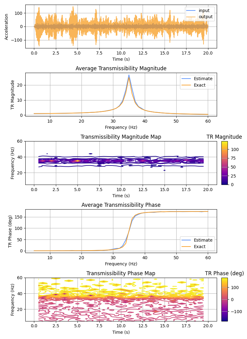
We’ll make up a pseudo-random signal with content from 5 to 60 Hz, and use that as a base-excitation (acceleration) input to a spring mass system. This is the same system as used in the pyyeti.srs.srs() routine:

  _____    ^
 |     |   |
 |  M  |  ---  SDOF response (x)
 |_____|
  /  |
K \ |_| C  ^
  /  |     |
[=======] ---  input base acceleration (sig)

We’ll then compute the transmissibility of the acceleration of the mass relative to the base-excitation. We should see a nice peak (roughly equal to the dynamic amplification factor Q) at the natural frequency of the single degree of freedom system. For the example, the frequency of the SDOF system is set to 35 Hz and Q is set to 25.

To check the results, the exact magnitude and phase from a closed-form frequency-domain solution (via pyyeti.ode.SolveUnc.fsolve()) will be plotted as well.

>>> import numpy as np
>>> import matplotlib.pyplot as plt
>>> from matplotlib import cm, colors
>>> import matplotlib.gridspec as gridspec
>>> from pyyeti import dsp, psd, ode
>>>
>>> # make up a flat (5-60 Hz) spectrum signal as input:
>>> psd_ = 1.0
>>> fstart = 5.0
>>> fstop = 60.0
>>> spec = np.array([[0.1, psd_], [100.0, psd_]])
>>> in_acce, sr, t = psd.psd2time(
...     spec, fstart, fstop, ppc=10, df=0.05, gettime=True,
...     winends={"ends": "both"}
... )
>>>
>>> # define a 35 hz system with 2% damping (Q = 25):
>>> frq = 35.0
>>> omega = frq * np.pi * 2
>>> Q = 25
>>> zeta = 1 / (2 * Q)
>>> ts = ode.SolveUnc(1, 2 * zeta * omega, omega ** 2, 1 / sr)
>>>
>>> # base-drive system like SRS ... in_acce is base input
>>> # (see pyyeti.srs.srs):
>>> #    zddot = input
>>> #    x = absolute displacement of mass
>>> #    u = x - z
>>> sol = ts.tsolve(-in_acce)
>>> out_acce = sol.a.ravel() + in_acce  # xddot
>>>
>>> tr = dsp.transmissibility(
...           in_acce, out_acce, sr, getmap=True)
>>>
>>> fig = plt.figure('Example', figsize=(8, 11), clear=True,
...                  layout='tight')
>>>
>>> # use GridSpec to make a nice layout with colorbars:
>>> gs = gridspec.GridSpec(5, 2, width_ratios=[30, 1])
>>>
>>> ax = ax_time = plt.subplot(gs[0, 0])
>>> _ = ax.plot(t, in_acce, label="input")
>>> _ = ax.plot(t, out_acce, alpha=0.75, label="output")
>>> _ = ax.set_xlabel("Time (s)")
>>> _ = ax.set_ylabel("Acceleration")
>>> _ = ax.legend(loc="upper right")
>>>
>>> # plot only frequency range where input has content:
>>> pv = (tr.f >= fstart) & (tr.f <= fstop)
>>> fm = tr.f[pv]
>>>
>>> # compute exact solution for comparison:
>>> in_acce_exact = np.ones(len(fm))
>>> sol = ts.fsolve(-in_acce_exact, fm)
>>> acce_exact = in_acce_exact + sol.a[0]
>>> mag_exact = abs(acce_exact)
>>> phase_exact = -np.angle(acce_exact, deg=True)
>>>
>>> # plot magnitude:
>>> ax = ax_freq = plt.subplot(gs[1, 0])
>>> _ = ax.plot(fm, tr.mag[pv], label="Estimate")
>>> _ = ax.plot(fm, mag_exact, label="Exact")
>>> _ = ax.set_xlabel("Frequency (Hz)")
>>> _ = ax.set_ylabel("TR Magnitude")
>>> _ = ax.set_title("Average Transmissibility Magnitude")
>>> _ = ax.legend(loc="upper right")
>>>
>>> ax = plt.subplot(gs[2, 0], sharex=ax_time)
>>> c = ax.contour(tr.t, fm, tr.mag_map[pv], 40,
...                cmap=cm.plasma)
>>> _ = ax.set_xlabel("Time (s)")
>>> _ = ax.set_ylabel("Frequency (Hz)")
>>> _ = ax.set_title("Transmissibility Magnitude Map")
>>>
>>> ax = plt.subplot(gs[2, 1])
>>>
>>> # This doesn't work in matplotlib 3.5.0:
>>> #   cb = fig.colorbar(c, cax=ax)
>>> #   cb.filled = True
>>> #   cb.draw_all()
>>> # But this does:
>>> norm = colors.Normalize(
...            vmin=c.cvalues.min(), vmax=c.cvalues.max()
...        )
>>> sm = plt.cm.ScalarMappable(norm=norm, cmap=c.cmap)
>>> cb = plt.colorbar(sm, cax=ax)  # , ticks=c.levels)
>>>
>>> _ = ax.set_title("TR Magnitude")
>>>
>>> # plot phase:
>>> ax = plt.subplot(gs[3, 0], sharex=ax_freq)
>>> _ = ax.plot(fm, tr.phase[pv], label="Estimate")
>>> _ = ax.plot(fm, phase_exact, label="Exact")
>>> _ = ax.set_xlabel("Frequency (Hz)")
>>> _ = ax.set_ylabel("TR Phase (deg)")
>>> _ = ax.set_title("Average Transmissibility Phase")
>>> _ = ax.legend(loc="lower right")
>>>
>>> ax = plt.subplot(gs[4, 0], sharex=ax_time)
>>> c = ax.contour(tr.t, fm, tr.phase_map[pv], 40,
...                cmap=cm.plasma)
>>> _ = ax.set_xlabel("Time (s)")
>>> _ = ax.set_ylabel("Frequency (Hz)")
>>> _ = ax.set_title("Transmissibility Phase Map")
>>>
>>> ax = plt.subplot(gs[4, 1])
>>>
>>> # This doesn't work in matplotlib 3.5.0:
>>> #   cb = fig.colorbar(c, cax=ax)
>>> #   cb.filled = True
>>> #   cb.draw_all()
>>> # But this does:
>>> norm = colors.Normalize(
...            vmin=c.cvalues.min(), vmax=c.cvalues.max()
...        )
>>> sm = plt.cm.ScalarMappable(norm=norm, cmap=c.cmap)
>>> cb = plt.colorbar(sm, cax=ax)  # , ticks=c.levels)
>>>
>>> _ = ax.set_title("TR Phase (deg)")

As an aside and for fun, compare the actual root-mean-square response to the Miles’ equation estimate. Miles’ should be a little higher on average … it assumes infinitely wide, flat input spectrum.

We’ll also compare the actual peak vs both:

• a 3 * sigma Miles’ peak

• a peak_factor * sigma Miles’ peak, where peak_factor is determined from the Rayleigh distribution

The Rayleigh peak factor is sqrt(2*log(duration*f)). See pyyeti.fdepsd.fdepsd() for the derivation of this factor. In this example, since the number of cycles is quite high, 3 sigma will generally be below the peak. The Rayleigh peak factor allows for a fairly good estimate of the actual peak.

>>> actual = np.sqrt((out_acce ** 2).mean())
>>> miles = np.sqrt(np.pi / 2 * Q * frq * psd_)
>>> if True:
...     print("rms comparison:")
...     print(f"\tactual        = {actual:.2f}")
...     print(f"\tMiles         = {miles:.2f}")
...     print(f"\tratio         = {actual/miles:.2f}")
rms comparison:
        actual        = 36.50
        Miles         = 37.07
        ratio         = 0.98
>>>
>>> # Compare actual peak to 3 sigma peak from Miles':
>>> actual_pk = abs(out_acce).max()
>>> miles_3s = 3 * miles
>>> if True:
...     print("peak comparison #1:")
...     print(f"\tactual        = {actual_pk:.2f}")
...     print(f"\t3 * Miles     = {miles_3s:.2f}")
...     print(f"\tratio         = {actual_pk/miles_3s:.2f}")
peak comparison #1:
        actual        = 134.00
        3 * Miles     = 111.22
        ratio         = 1.20
>>>
>>> rpf = np.sqrt(2 * np.log(frq * t[-1]))  # rayleigh peak factor
>>> miles_rayleigh = rpf * miles
>>> if True:
...     print("peak comparison #2:")
...     print(f"\tactual        = {actual_pk:.2f}")
...     print(f"\t{rpf:.2f} * Miles  = {miles_rayleigh:.2f}")
...     print(f"\tratio         = {actual_pk/miles_rayleigh:.2f}")
peak comparison #2:
        actual        = 134.00
        3.62 * Miles  = 134.19
        ratio         = 1.00